Stochastic Analysis of a System with Preventive
Maintenance and Common Cause Failure
Khaled M. El-Said
Department of Mathematics, Faculty of Science, Helwan University P. O. Box 11795, Cairo, Egypt
ABSTRACT
This paper Study the reliability and availability characteristics of the system with PM and CCF. The failure times , replacement times, PM times and CCF times of a components are assumed to be exponentially distributed. We derive the mean time to failure( MTTF) and the steady state availability( ) in this system. Some Special cases have been studies theoretically and graphically to observe the effect of the preventive maintenance (PM) and Common Cause Failure (CCF) on system performance. Certain important results have been derived as special cases.
Keywords
Mean Time to System Failure (MTSF), Steady-state availability, Preventive Maintenance (PM) and the Kolmogorov’s forward equations method, Common Cause Failure (CCF).
1.
INTRODUCTION
Several authors [1, 3, 4, 5, 7, 8] studied the reliability analysis of different behaviors' systems. Goel & Shrivastava [6] studied comparison reliability characteristics of two systems with bivariate exponential lifetimes. Sing and Rawal [9] studied the availability analysis of series system with human failure under different repair policies. Researchers in reliability have shown a keen interest in the analysis of two (or more) component parallel systems owing to their practical utility in modern industrial and technological set-ups. In these systems, more commonly used are those in which the failure in one component affects the failure rates of other components. For example we can consider engine failure in two engine planes, wear of two pens on an executive's desk or the performance of individual's eyes, ears, kidneys and other paired physical organs. A CCF is defined as the failure of single unit or multiple units due to a single common-cause. Some of the CCF may occur due to the following reasons. 1- Wrong designing of equipment during design phase. 2- Improper maintenance of machines by workers. 3- Natural catastrophe likes flood, earthquake, fire… etc. 4- High temperature of computer chips.
The purpose of this study is to study the system with two dissimilar components arranged in parallel with Preventive Maintenance (PM) and Common Cause Failure (CCF). We analyzed the system by using Kolmogorov,s forward equation method.
We derived measures of system effectiveness like MTSF and the steady-state availability . Graphical Studies of effect the Preventive Maintenance (PM) and Common Cause Failure (CCF) on the measures mentioned above are also given.
2. Material and Method
In this study, the system is analyzed by using Kolmogorov , s equations method. Various measures of system effectiveness such mean time to system failure MTSF and Steady State Availability in this system has been obtained.
1
The failure rate of component A1
The failure rate of component B2
The failure rate of component A when B has already failed2
The failure rate of component B when A has already failed
The replacement rate of component A
The replacement rate of component B
The replacement rate of component A , B
The rate of time for taking a unit into preventive maintenance The preventive maintenance rate
The CCF of unit A.
The CCF of unit B.)
(
t
P
i Probability the components are working at time,
t
(
t
0
)
at stateS
iN
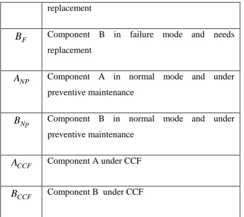
A
Component A in normal mode and operativeN
B
Component B in normal mode and operativereplacement
F
B
Component B in failure mode and needs replacementNP
A
Component A in normal mode and under preventive maintenanceNp
B
Component B in normal mode and under preventive maintenanceCCF
A
Component A under CCFCCF
B
Component B under CCFAssumptions
1-The system consists of a single unit having two dissimilar parallel
Components, say A and B.
2- The system remains operative even if a single component operates.
3- The failure of a component changes the life time parameter of the other.
4- Each component can be replaced with a similar component with both the Components (when failed) can also be replaced simultaneously
5- After replacement of each component, the system is as good as new.
6- CCF and other failures are statistically independent.
7- CCF, other failure, replacement and preventive maintenance rates are constant.
8- Preventive maintenance (e.g. overhaul, inspection, minor repairs, etc.)
A unit can be in one of the following states at time t is
Up States :
)
,
(
0
A
NB
NS
,S
1
(
A
F,
B
N)
,S
2
(
A
N,
B
F)
,) , (
4 ANp BNp
S
Down States :
S
4
(
A
F,
B
F)
,S
5
(
A
CCF,
B
CCF)
Table (1):- Transition rates
S0 S1 S2 S3 S4 S5
S0 1 1
S1 2
S2 2
S3
S4
S5
2.
Mean time to system failure
From table (1) above, Let
P
i(
t
)
to be the Probability thatthe system at time t
(
t
0
)
is in stateS
i. LetP
(
t
)
be the probability row vector at time t, we have the following initial condition.
(
0
),
(
0
),
(
0
),
(
0
),
,
(
)
1
,
0
,
0
,
0
,
0
,
0
)
0
(
P
0P
1P
2P
3P
4P
5t
P
We obtain the following differential equations
),
(
)
(
)
(
)
(
)
(
)
(
)
(
)
(
1 1 0 1 2 3 4 5 0t
P
t
P
t
P
t
P
t
P
t
P
t
P
),
(
)
(
)
(
)
(
1 0 2 11
t
P
t
P
t
P
),
(
)
(
)
(
2 2 01
2
P
t
P
t
P
),
(
)
(
)
(
0 33
t
P
t
P
t
P
),
(
)
(
)
(
)
(
2 1 2 2 4 4t
P
t
P
t
P
t
P
).
(
)
(
)
(
0 5 5t
P
t
P
t
[image:2.595.48.289.70.284.2], QP P (2) Where,
0 0 0 0 0 0 0 0 0 0 0 0 0 0 ) ( 0 0 0 0 0 ) ( ) ( 2 2 2 1 2 1 1 1 QIt is difficult to evaluate the transient solutions hence we delete the rows and columns of absorbing state of matrix Q and take the transpose to produce a new matrix, say A.
The expected time to reach an absorbing state is obtained from 1 1 1 1 ) )( 0
( A 1
P
MTSF (3)
Where,
0 0 0 ) ( 0 0 0 ) ( ) ( 2 2 1 1 1 1 AWe obtain the MTSF of the form
] [
] [
2K G Z K L MTSF
(4) Where, )} ( ){ ( ), )( ( ), )( ( ), ( 1 2 2 2 2 1 2 2 2 1
G L Z K4. Availability analysis
For the availability case of table (1), using the same initial conditions
(
0
),
(
0
),
(
0
),
(
0
),
(
0
),
(
0
)
1
,
0
,
0
,
0
,
0
,
0
)
0
(
P
0P
1P
2P
3P
4P
5
P
The differential equations above can be expressed as
) ( ) ( ) ( ) ( ) ( ) ( 0 0 0 0 0 0 0 0 0 0 0 0 0 0 ) ( 0 0 0 0 0 ) ( ) ( ) ( ) ( ) ( ) ( ) ( ) ( 5 4 3 2 1 0 2 2 2 1 2 1 1 1 5 4 3 2 1 0 t P t P t P t P t P t P t P t P t P t P t P t P
The system availability can be obtained from the solutions for Pi(t), i =0,1,2,…5.The states 0,1,2,3 in table(1) are the only up
sates of the system. The steady-state availability is given by
)]
(
)
(
[
1
)
(
P
0
P
1
P
2
P
3
P
4
P
5
A
(5)In the steady state, the derivatives of the state probabilities become zero so that
,
0
)
(
P
Q
(6)Which in matrix form
0 0 0 0 0 0 ) ( ) ( ) ( ) ( ) ( ) ( 0 0 0 0 0 0 0 0 0 0 0 0 0 0 ) ( 0 0 0 0 0 ) ( ) ( 5 4 3 2 1 0 2 2 2 1 2 1 1 1 P P P P P P
The following normalizing condition
1
)
(
)
(
)
(
)
(
)
(
)
(
1 2 3 4 50
P
P
P
P
P
P
(7) 1 0 0 0 0 0 ) ( ) ( ) ( ) ( ) ( ) ( 1 1 1 1 1 1 0 0 0 0 0 0 0 0 0 0 ) ( 0 0 0 0 0 ) ( ) ( 5 4 3 2 1 0 2 2 2 1 2 1 1 1 P P P P P P
The system of equations in matrix above to obtain the steady-state probabilities
)
(
),
(
5 4
P
P
The steady state availability is given by
}] ) ( ) ( { [ ) ( ( ) ( 2 1 2 2 Z K L L Z K L A
(8)5. Special Cases
5.1 Study the system without preventive
maintenance
The mean time to system failure is given by
MTSF1 =
G K Z K 2
The steady state availability is given by
Z K L Z K A
) ( ) ( ) ( ) ( 2 1 2 2 15.2 Study the system without Common Cause
Failure
The results of Ref. [2] are derived.
5.3 Study the system without preventive
maintenance and Common Cause Failure
The results of Ref. [2] are derived.
6. Graphical Study
The purpose of this section studies the effect of (PM) on the system. The following numerical results are obtained by considering the following system parameters:- We fix
05
.
0
,
4
.
0
,
4
.
0
,
3
.
0
,
05
.
0
,
3
.
0
,
2
.
0
21
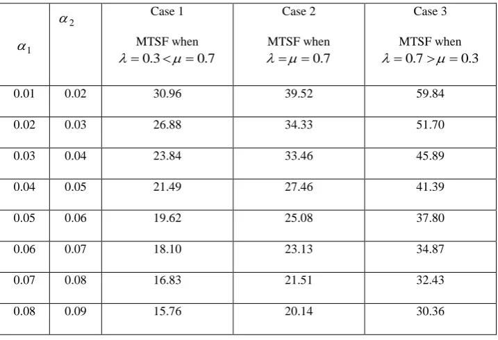
Table (2) :- The mean time to system failure MTSF by using three cases of PM.
1
2
Case 1MTSF when 7 . 0 3 .
0
Case 2 MTSF when 7 . 0
Case 3 MTSF when 3 . 0 7 .0
0.01 0.02 30.96 39.52 59.84
0.02 0.03 26.88 34.33 51.70
0.03 0.04 23.84 33.46 45.89
0.04 0.05 21.49 27.46 41.39
0.05 0.06 19.62 25.08 37.80
0.06 0.07 18.10 23.13 34.87
0.07 0.08 16.83 21.51 32.43
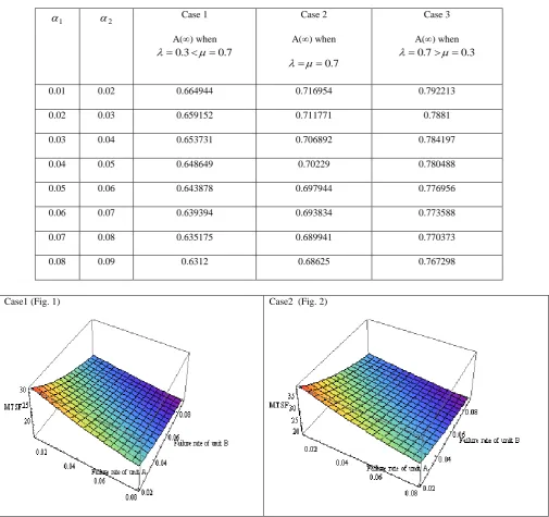
[image:4.595.119.478.476.721.2]Table (3):- The steady-state availability A () by using three cases of PM.
1
2 Case 1A() when
7 . 0 3 .
0
Case 2
A() when
7 . 0
Case 3
A() when
3 . 0 7 .
0
0.01 0.02 0.664944 0.716954 0.792213
0.02 0.03 0.659152 0.711771 0.7881
0.03 0.04 0.653731 0.706892 0.784197
0.04 0.05 0.648649 0.70229 0.780488
0.05 0.06 0.643878 0.697944 0.776956
0.06 0.07 0.639394 0.693834 0.773588
0.07 0.08 0.635175 0.689941 0.770373
0.08 0.09 0.6312 0.68625 0.767298
[image:5.595.50.556.101.576.2]Case3 (Fig. 3) Case 1 (Fig. 4)
Case2 (Fig.5) Case3 (Fig.6)
3.
CONCLUSION
We used computer software, to compare MTSF under effect of (PM). This result show that
MTSF in (Case1) < MTSF in (Case2) < MTSF in (Case3) and
A ()in (Case1) < A ()in (Case2) < A () in (Case3)
We conclude that the system after adding of preventive maintenance (PM). The system has the high reliability, in (case3).
4.
ACKNOWLEDGMENTS
5.
The author is thankful to the reviewers for their constructive comments which have helped to improve the manuscript.6.
REFERENCES
[1] El-Said, Kh. M., (2008), "Cost analysis of a system with preventive maintenance by using Kolmogorov,s forward equations method", Ame. J. of App. Sci. 5(4), 405 - 410. [2] El-Said, Kh. M., and Moh. S. El - Sherbeny, (2005), "Evaluation of reliability and availability characteristics of two different systems by using linear first order differential equations", J. Math. and Stat., 1(2), 119 - 123.
catastrophic failures and preventive maintenance ", Microelectron. Reliab., Vol.24, No.5,881 – 883.
[5] GOEL, L. R., SHARMA,G.C. and GUPTA, P., (1986), " Reliability analysis of a system with preventive maintenance inspection and two types of repair", Microelectron. Reliab., Vol.26, No.3,429 – 433.
[6] GOEL, L. R. and SHRIVASTAVA, P., (1992), "Comparison of reliability characteristics of two (double component) systems with bivariate exponential lifetimes ", Int. J. Systems Sci, Vol.23, No.1,135 – 144.
[7] GOPALAN, M. N. and NAGARWALIA, H.E., (1985),"Cost benefit analysis of a one – server two – unit
cold standby system with repair and preventive maintenance ", Microelectron. Reliab. Vol.25, No.2,267 – 269.
[8] Kuo - Hsiung Wang , Ching-Chang Kuo., (2000), " Cost and probabilistic analysis of series systems with mixed standby components ", Applied Mathematical Modelling, Vol. 24, 957 –967.