New Programming Approach for Steepest Descent Optimization of Rocket Trajectories

ABSTRACT

In this paper a new programming methodology for optimizing rocket trajectories using steepest descent technique is presented. The programming is done in Matlab platform. At first the dynamical equations of rocket is derived and for the proper derivation and analysis of the equations ,Eulers integration method is used. A new programming approach is designed and the equations are optimized using steepest descent technique, assuming certain boundary conditions. The results obtained are verified and it is seen that the optimal trajectory is attained with all objectives satisfied. This project is done at Vikram Sarabhai Space Centre(VSSC),a constituent of Indian Space Research Organization(ISRO).

General Terms

Rocket dynamics,Euler‟smethod,Simulator program.

Keywords

Rocket trajectory,Matlab,Optimization,Steepest descent

1.

INTRODUCTION

The optimality of rocket trajectories may be defined according to several objectivesliketransfer time is minimal for a given propellant and payload mass (i.e. for a given launch mass),the required propellant mass is minimal for a given transfer time and launch mass, the required propellant mass is minimal for a given transfer time and payload mass.In practice, the methods of solving deterministic optimal control problems are divided into two categories: direct and indirect methods[9]. Indirect methods proceed by formulating the optimality conditions according to the Pontryagin maximum principle and then numerically solving the resulting two point boundary value problem. Direct methods discretize the original problem in time and solve the resulting parameter optimization problem and thus generate an approximate solution of the original problem. Both methods solve the necessary conditions of optimality and both discretize the problem. The most common objective is to minimize the propellant required or equivalently to maximize the fraction of the rocket that is not devoted to propellant. Of course, as is common in the optimization of continuous dynamical systems, it is usually necessary to provide some practical upper bound for the final time or the optimizer will trade time for propellant. There are also rocket trajectory problems where minimizing flight time is an important, or, for example those using continuous thrust, where minimizing flight time and minimizing propellant use are synonymous.

2.

MATHEMATICAL

REPRESENTATION OF

ROCKETDYNAMICS

Point-mass equations of motion with non-rotating

sphericalearth are considered in this paper, which is given by

𝑟 = 𝑉𝑠𝑖𝑛𝛾 (1)

𝑉 = 1

𝑚𝑉 𝑇 𝑐𝑜𝑠𝛼 − − 𝑚𝑔 𝑠𝑖𝑛𝛾 (2)

𝛾 = 1

𝑚𝑉 𝑇 𝑠𝑖𝑛𝛼 + 𝑉 𝑟−

𝑔

𝑉 𝑐𝑜𝑠𝛾 (3)

For a problem without path constraints, with terminal equality constraints, and with an initial state vector whose components are either fixed or optimizable, the first order necessary conditions can be formulated as shown in equations from 4 to(11).

Hamiltonian:

𝐻 = 𝐿 + 𝜆𝑇_{𝑓 (4)}

Dynamics:

𝑋 = 𝑓 𝑥, 𝑢, 𝑡 = (𝜕𝐻

𝜕𝜆)𝑇 (5)

Adjoint differential equations:

𝜆 = (𝜕𝐿 𝜕𝑥)𝑇− (

𝜕𝑓 𝜕𝑥)𝑇𝜆 = (

𝜕𝐻

𝜕𝑥)𝑇 (6)

Optimality condition:

(𝜕𝐻

𝜕𝑢)𝑇 = 0 = ( 𝜕𝑓 𝜕𝑢)𝑇𝜆 + (

𝜕𝐿

𝜕𝑥)𝑇 (7)

Initial conditions:

𝑥𝑘(𝑡0)given or 𝜆𝑘 𝑡0 = 0 (8)

Terminal constraints:

𝛹𝑓 𝑥𝑓, 𝑡𝑓 = 0 (9)

New Programming Approach for Steepest Descent

Optimization of Rocket Trajectories

Vishnu G Nair

Department of Aeronautical & Automobile Engineering, Manipal Institute of Technology

Manipal, India-576104

Dileep M V

Department of Instrumentation & Control Engineering, Manipal Institute of Technology

Manipal, India-576104

Prahalad K R

Department of Instrumentation & Control Engineering, Manipal Institute of Technology

Transversality conditions:

𝜆𝑓 = (𝜕∅_𝜕𝑥+ 𝑣𝑇

𝜕𝛹𝑓

𝜕𝑥)𝑡=𝑡𝑓 (10)

Transversality condition for optimizable𝑡𝑓:

Ω= [(𝜕∅ 𝜕𝑡+ 𝑣𝑇

𝜕𝛹𝑓

𝜕𝑡 + 𝐻)]𝑡=𝑡𝑓 (11)

Where L = Lagrangefunction

H = Hamilton function

𝜆 = costate variable

Euler-Lagrange [22] equations were extended by the introduction of further necessary conditions, such as the Legendre- Clebsch condition, The Jacobi condition[4] and the Weierstrass condition[4].

𝜕2_𝐻

𝜕𝑢2 ≥ 0 (12)

A detailed discussion on these conditions can be found in Ref. [22].In this part optimization of the three variables take place, they are radial distance from the center of earth 𝑟, rocket velocity 𝑣 and the flight path angle 𝛾.The equations 1 − (3) can be described in generic form as,

𝑋 = 𝑓 𝑋, 𝑈 (13)

𝑟 𝑣 𝛾 =

𝑉𝑠𝑖𝑛𝛾 1

𝑚𝑉(𝑇𝑐𝑜𝑠𝛼 − 𝑚𝑔𝑠𝑖𝑛𝛾 ) 1

𝑚𝑉 (𝑇𝑠𝑖𝑛𝛼 ) + ( 𝑉 𝑟−

𝑔 𝑉) 𝑐𝑜𝑠𝛾

(14)

Where the state and control vectors are defined as

𝑋 = 𝑥1𝑥2𝑥3𝑇 (15)

That is

𝑋 = 𝑟𝑣𝛾 𝑇 ₍₁₆₎

𝑈 = 𝛼 (17)

In this a trajectory optimization problem of a single stage launch vehicle is considered. The objective here is to generate the guidance command history 𝛼 𝑡 , 𝑡 ∈ 𝑡0, 𝑡𝑓 such that the

following concerns are taken care of,

(a) At the final time 𝑡𝑓, the specified terminal constraints must

meet as accurately. The terminal constraints include constraints on altitude, velocity and flight path angle (which is the angle made by the velocity vector with respect to the local horizontal).

(b) The system should demand minimum guidance command, which can be ensured by formulating a „minimum time‟ problem.

To achieve the above objectives, the following cost function is selected, which consists of terminal penalty terms and a dynamic control minimization term.

𝐽 = (𝑟 𝑡𝑓 − 𝑟𝑓)2𝑠𝑟+ (𝑣 𝑡𝑓 − 𝑣𝑓)2𝑠𝑣

+ (𝑟𝑜𝑤 𝑡𝑓 − 𝑟𝑜𝑤𝑓)2𝑠𝛾 (18)

Where 𝑠𝑟,𝑠𝑣,𝑎𝑛𝑑𝑠𝛾 weighing factors. The Hamiltonian (Ref equation (4)) is defined as ,

𝐻 = 𝐽 + 𝜆𝑇 ₍₁₉₎

Where 𝜆𝑇= [𝜆1𝜆2𝜆3], costate variables.

𝐻 = 𝐽 − 𝜆1 𝑉𝑠𝑖𝑛𝛾 − 𝜆2 _𝑚𝑉1 𝑇𝑐𝑜𝑠𝛼 − 𝑚𝑔𝑠𝑖𝑛𝛾

− 𝜆3 _𝑚𝑉1 𝑇𝑠𝑖𝑛𝛼 𝑉_𝑟

−𝑔

𝑉 𝑐𝑜𝑠𝛾 (20)

From equation (18) we get

𝐻 = (𝑟 𝑡𝑓 − 𝑟𝑓)2𝑠𝑟+ (𝑣 𝑡𝑓 − 𝑣𝑓)2𝑠𝑣

+ (𝑟𝑜𝑤 𝑡𝑓 − 𝑟𝑜𝑤𝑓)2𝑠𝛾− 𝜆1 𝑉𝑠𝑖𝑛𝛾

− 𝜆2 _𝑚𝑉1 𝑇𝑐𝑜𝑠𝛼 − 𝑚𝑔𝑠𝑖𝑛𝛾

− 𝜆3 _𝑚𝑉1 𝑇𝑠𝑖𝑛𝛼

+ 𝑉 𝑟−

𝑟

𝑉 𝑐𝑜𝑠𝛾 (21)

Equation (21) gives the final Hamiltonian function. This function has solve to get the optimum solution .Therefore

𝜕𝐻 𝜕𝑟= 𝜆3

𝑣

𝑟2𝑐𝑜𝑠𝛾 = −𝜆1 (22)

𝜕𝐻

𝜕𝑣= −𝜆1𝑠𝑖𝑛𝛾 + 𝜆3− 1

𝑚𝑣2 𝑇𝑠𝑖𝑛𝛼 −

1 𝑟−

𝑔 𝑣2 𝑐𝑜𝑠𝛾

= −𝜆2 (23)

𝜕𝐻

𝜕𝛾= −𝜆1𝑐𝑜𝑠𝛾 − 𝜆2𝑔𝑐𝑜𝑠𝛾+ 𝜆3 𝑣 𝑟−

𝑔 𝑣 𝑠𝑖𝑛𝛾

= −𝜆3 (24)

𝜕𝐻 𝜕𝛼= 𝜆2

𝑇

𝑚𝑠𝑖𝑛𝛼 − 𝜆3 𝑇

𝑚𝑣𝑐𝑜𝑠𝛼 (25)

The above equations 22 − 25 to be solved to get the solutions of costate variables, that is 𝜆1, 𝜆2𝑎𝑛𝑑𝜆3. In an

conditions. The equations 1 2 & 3 in the simulator program is developed initial steering profile for steepest descent optimization is obtained.For finding the accurate steering profile taking an assumption that is acceleration is a linearly increasing quantity. So rate of change of velocity is approximating as linear function. This linear function is selected by polynomial approximation[17] that is by changing the functions randomly to fit the curve properly.

𝛼 = 𝑐𝑜𝑠−1 𝑐1𝑡 + 𝑐2+ 𝑔 𝑠𝑖𝑛𝛾

𝑇 𝑚 (26)

Now knowing the values of 𝜆1 , 𝜆 𝑎𝑛𝑑𝜆2 3 , so to get

𝜆1, 𝜆2𝑎𝑛𝑑𝜆3 have to integrate. Therefore the final values of

𝜆𝑇_{is 𝜆}

1𝑓, 𝜆2𝑓𝑎𝑛𝑑𝜆3𝑓. To find the final values of 𝜆.

𝜆1𝑓=𝜕𝐽_𝜕𝑟= 2 × 𝑠𝑟× 𝑟 𝑡𝑓 − 𝑟𝑓 (27)

𝜆2𝑓=_𝜕𝑣𝜕𝐽= 2 × 𝑠𝑣× 𝑣 𝑡𝑓 − 𝑣𝑓 (28)

𝜆3𝑓=_𝜕𝛾𝜕𝐽= 2 × 𝑠𝛾× 𝛾 𝑡𝑓 − 𝛾𝑓 (29)

The integration method used in the optimal control problem is Eulers method. It is the usual basic method.

2.1Implementation of Euler’s method

Euler‟s method can be implemented both in simulator program and the optimal control problem. In simulator program the integration of 𝑟, 𝑣 𝑎𝑛𝑑 𝛾 happens. That is given as follows.

𝑟 = 𝑟0+ 𝑟 𝑑𝑡 (30)

𝑣 = 𝑣0+ 𝑣 𝑑𝑡 (31)

𝛾 = 𝛾0+ 𝛾 𝑑𝑡 (32)

In optimal control the 𝜆𝑇 is integrating to get final 𝜆 values.

𝜆1= 𝜆10+ 𝜆1 𝑑𝑡 (33)

𝜆2= 𝜆20+ 𝜆2 𝑑𝑡 (34)

𝜆3= 𝜆30+ 𝜆3 𝑑𝑡 (35)

Where 𝑑𝑡 is the integration step size.𝑟0, 𝑣0&𝛾0are the initial

values of 𝑟, 𝑣 𝑎𝑛𝑑 𝛾. Similarly 𝜆10, 𝜆20&𝜆30are the initial values of 𝜆1, 𝜆2&𝜆3 .Thus gets the solution of equation

(21)For optimal solutions, The optimality condition (Ref equation (26)) is given by

𝜕𝐻

𝜕𝛼= 0 (36)

The weighting factor tow (𝜏) should select according to the steepest descent method . That is

𝑡𝑜𝑤𝑤 =𝜕𝐻 𝜕𝛼×

𝜕𝐻 𝜕𝛼

𝑇

(37)

tow 𝜏 = 1 𝑡𝑜𝑤𝑤

2 (38)

Thus weighting factor tow (𝜏) is obtained. Then it is applied to the control variable alpha (𝛼) ,toget the new alphaprofile.

𝛼 = 𝛼0−

𝜕𝐻

𝜕𝛼× tow 𝜏 (39)

Where 𝛼0= privious computed 𝛼

Equation 21 is the gradiant function, optimizes the objective function. An optimal control problem needs accurate initial conditions. From the equations 1 − (3) the simulator program is developedand initial steering profile for steepest descent optimization is obtained.For finding the accurate steering profile acceleration is assumed to be a linearly increasing quantity. So rate of change of velocity is approximated as linear function. This linear function is selected by polynomial approximation that is by changing the functions randomly to fit the curve properly. The vehicle acceleration is a linear function of time as given in the equation. The constants are obtained by varying initial and final steering angle value. Thus tuning of constants𝑐1 𝑎𝑛𝑑 𝑐2are done. The initial and final 𝛼 is thus obtained to be3.5 𝑑𝑒𝑔⁡and 14 𝑑𝑒𝑔 respectively.Therefore by solving the equation 21 using the initial and final values the appropriates values for 𝑐1 𝑎𝑛𝑑 𝑐2 can be find out;

𝑐1= 6.4217 × 10−3

𝑐2= 1.918235

3

SIMULATOR PROGRAM STEPS AND

RESULTS

The simulator program is mainly used for generating the initial steering angle. This steering is given as the input thrust angle for trajectory optimization problem. Table (1)shows travelling time and the initial steering angle profile. The main programming steps are given below:-

a)-Develop rocket dynamics equations.

b)-To get initial alpha profile develop a simulator program that has minimum objective function values.

c)-Put this alpha profile in the trajectory optimization problem.

e)Alpha profile is updated by using steepest descent technique.

f) Alpha profile update is done by tuning of multiplication factor.

g) The optimized result will be obtained after 82 iterations.

The results obtained are shown below:-

Table 1 Travelling time and the initial steering angle profile

Time in seconds

initial thrust angle

𝛼 values in radian

1 0.275101

50 0.279912

100 0.271316

150 0.255160

200 0.235788

250 0.217232

300 0.203625

350 0.198925

400 0.206037

450 0.226118

500 0.258920

510 0.266945

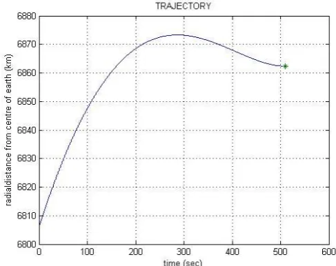
Figure 1 shows the graph obtained for the simulation program.The figure indicates the radial distance from earth centre.The symbol,„ * ‟ indicates the target, 𝑟𝑓 = 6862.41573 𝑘𝑚. By this method, the rocket achieved the desired position, but not the desired velocity. Therefore the above method is not an optimized one. So has to be optimized.

Fig 𝟏 Radial distance from earth centreVs time

Fig 𝟐 Velocity Vs time

Fig 𝟑: Flight path angle Vs time

Figure 3 & (2) indicates the flight path angle and velocity variation with respect to time.1n figure (4.8), the symbol‘ ∗ ’

and in figure 3 , it indicates the value of final gamma, 𝛾 =

0 𝑑𝑒𝑔. In figure (2) the desired target-velocity is not achieved. The simulation program provides the basic model trajectory and the initial steering angle. The trajectory optimization problem is explained in the following sections. Euler‟s method of integration can be used for optimization. In Euler‟s method of integration the integration step size is same. Iteration results are shown below. Total iteration number =

82

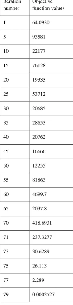
Table 2 Itration number and the objective function value

Iteration number

Objective function values

1 64.0930

5 93581

10 22177

15 76128

20 19333

25 53712

30 20685

35 28653

40 20762

45 16666

50 12255

55 81863

60 4699.7

65 2037.8

70 418.6931

71 237.3277

73 30.6289

75 26.113

77 2.289

79 0.0002527

80 8.3802× 10−6

81 0.0002527

82 8.3802× 10−6

Table (2) shows the objective function values for each iteration. By analyzing the objective function values, it seems to be decreasing and tends to a minimum value. Table (3) shows final radial distance from center of earth, final velocity of rocket and final flight path angle in each iteration.

Table 3 Iterationnumber, final radial distance, final velocity and final flight path angle

Iteration number

final radial distance from centre of earth

(𝑘𝑚)

final velocity of rocket

(𝑚/𝑠)

Final flight path angle (𝑟𝑎𝑑)

1 6862.4 7703.6 0.0002116

5 68655 7696.6 0.0015444

10 6863.9 7700.7 -0.0002827

15 6865.2 7697.5 -0.0004971

20 6863.8 7700.2 -0.0024106

25 6864.7 7696.5 -0.0030378

30 6863.9 7696.0 -0.0049032

35 6864.1 7691.4 -0.0061224

40 6863.9 7686.7 -0.0076483

45 6863.7 7680.5 -0.0090698

50 6863.5 7673.3 -0.010482

55 6863.3 7664.9 -0.011885

60 6863.1 7655.5 -0.013288

65 6862.9 7645.0 -0.014698

70 6862.6 7633.5 -0.016121

71 6862.6 7631.0 -0.016407

73 6862.5 7626.1 -0.016981

77 6862.4 7623.6 -0.017293

79 6862.4 7623.5 -0.017286

80 6862.4 7623.5 -0.017286

81 6862.4 7623.5 -0.017286

82 6862.4 7623.5 -0.017286

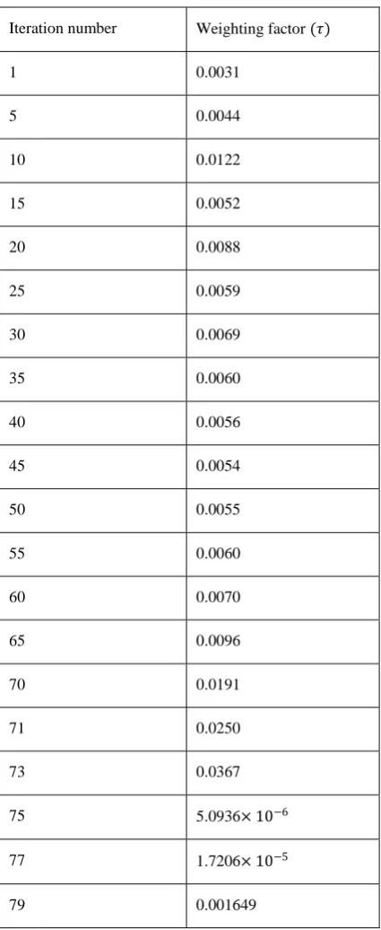
Table 4 Itration number and weighting factor (𝝉)

Iteration number Weighting factor (𝜏)

1 0.0031

5 0.0044

10 0.0122

15 0.0052

20 0.0088

25 0.0059

30 0.0069

35 0.0060

40 0.0056

45 0.0054

50 0.0055

55 0.0060

60 0.0070

65 0.0096

70 0.0191

71 0.0250

73 0.0367

75 5.0936× 10−6

77 1.7206× 10−5

79 0.001649

80 0.011844

81 0.001649

82 0.011843

Table (4) shows weighting factor (𝜏) variation in each iteration. Weighting factor has a significant major role in optimizing the trajectory. Figure 4 , (5) & (6) shows the graphs obtained for Steepest Descent method with Euler‟s integration. The figure (4)indicates the radial distance from

earth center. The symbol, „ * ‟ indicates the target,𝑟𝑓 =

6862415.73 𝑚 . The above method is optimized with minimum objective function value. From the graph it can be

seen that the rocket achieved the target-position .A higher altitude is considered in this method, sothat it can achieve the

target-velocity.

Fig.𝟒 Radial distance from the centre of earth Vs time

Figure 5 &(6)indicates the flight path angle and velocity variation with respect to time.1n figure 5 the symbal‘ ∗ ’ indicate the final velocity, 𝑉𝑓 = 7623.5321 𝑚/𝑠 and in figure 6 the symbal‘ ∗ ′ indicates final gamma , 𝛾 =

Fig 5 VelocityVstime

Fig .6 Flight path angle Vs time

5 .CONCLUSIONS

A new programming approach for steepest descent optimization of rocket trajectories is presented in this paper. From the results it is clear that the final objectives are achieved with optimum resources and time. All the constraints are satisfied and the trajectory is a optimal one. This methodology can be implemented in future missions and the results ]can be verified and compared with the real time outputs. Comparison of the results with real time results and formulation of more efficient algorithms will be the future work.

6 .ACKNOWLEDGMENTS

The authors would like to express their appreciation to Dinesh Kumar, Scientist grade D ,of Indian Space Research Organization (ISRO) for his sensible help and honourable support.

7 .REFERENCE

[1]John T. Betts “Survey of Numerical Methods for Trajectory Optimization”, AIAA Journal of Guidance, Control and Dynamics, Vol. 21, No. 2, March-April 1998, pp. 193-207.

[2] Betts, J. T., and Frank, P. D., “A Sparse Nonlinear Optimization Algorithm,” Journal of Optimization Theory and Applications, Vol. 82, 1994, pp. 519–541. [3]Peter F. Gath, Klaus H. Well “Trajectory Optimization

Using A Combination of Direct Multiple Shooting”AIAA Guidance, Navigation, and Control Conference and Exhibit 6-9 August 2001 Montreal, Canada.

[4]Peter Friedrich Gath “CAMTOS - A Software Suite Combining Direct and Indirect Trajectory Optimization Methods” Institute of Flugmechanik und Flugregelung University Stuttgart 2002.

[5]LukkanaVaraprasad and RadhakantPadhi “Ascent Phase Trajectory Optimization Of a Genetic Launch Vehicle ” XXXII NATIONAL SYSTEMS CONFERENCE, NSC 2008, December 17-19, 2008

[6]JukkaRanta“optimal control and flight trajectory optimization applied to evasion analysis”Espoo, March 2004

[7]Siddal, J.N.,“ Optimal Engineering Design: Principles and Applications”, Mercell Dekker Inc., New York, NY, 1982.

[8]Bryson, A. E. and Denham, W. F., “A Steepest-Ascent Method for Solving Optimum Programming Programs,” Journal of Applied Mechanics, Vol. 29, pp. 247-257, June 1962.

[9]Fletcher, R., “Practical Methods of Optimization,” Vol. 2, ConstrainedOptimization,Wiley, New York, 1985. [10]Gilberto E. Urroz, “Solution of non-linear equations”

September 2004

[11]Bruce A. Conway “Spacecraft Trajectory Optimization”Cambridge University Press, © Cambridge University Press 2010ISBN-13 978-0-521-51850-5

[12]Donald Greenspan “ Numerical Solution of Ordinary Differential Equations for Classical, Relativistic and Nano Systems. ” Copyright © 2006 WILEY-VCH Verlag GmbH & Co. KGaA, Weinheim, ISBN: 3-527-40610-7

[13]Ulrich Walter“Astronautics” © 2008 WILEY-VCH Verlag GmbH & Co. KgaA,Weinheim ISBN:978-3-527-40685-2 [14]Mischa Kim“Continuous Low-Thrust Trajectory

Optimization: Techniques And Application” © 2005 by Mischa Kim

[15]Desineni Rama Naidu “Optimal control Systems”Boca Raton London New York Washington, D.C. © 2003 by CRC Press LLC ISBN 0-8493-0892-5

[16]Bryson, A.E., Jr., Ho, Y.-C., “Applied Optimal Control”, Revised Printing, Hemisphere Publishing Corporation, 1975

[17]Gordon K. Smyth “Polynomial Approximation”John Wiley & Sons, Ltd, Chichester, 1998 ,ISBN 0471 975761 [18]John H. Mathews and Kurtis K. Fink “Numerical Methods

Using Matlab ”, 4th Edition, 2004ISBN: 0-13-065248-2 [19]“THE ART OF SCIENTIFIC COMPUTING ”Copyright