A Comparative Study of Assessing Software Reliability using SPC: An MMLE Approach

(1)

23

A Comparative Study of Assessing Software

Reliability using Spc: an Mmle Approach

Bandla.Srinivasa Rao

Department of Computer

Science and Engineering

VRS & YRN College of

Engineering and Technology

Chirala, India

R.Satya Prasad

Phd,Department of Computer

Science and Engineering

Acharya Nagarjuna

University

Guntur, India

K. Ramchand H Rao

Phd,Department of Computer

Science and Engineering

A.S.N. Womens Eng.College

Tenali, India

ABSTRACT

The Modified Maximum Likelihood Estimation (MMLE) of the parameters of Exponential and Half Logistic distributions are considered and compared. An analytical approximation is used instead of linear approximation for a function which appears in Maximum Likelihood equation. These estimates are shown to perform better, in the sense of simplicity of calculation than the one based on linear approximation for the same function. In this paper we identified the MMLE method of estimations and associated results using Half Logistic Distribution and Exponential Distribution are similar. These estimates are used in SPC to find the control limits to predict the software reliability. A comparison of software reliability using Statistical Process Control for a small sample is also presented

Key words

Software Reliability, Statistical Process Control, Modified Maximum Likelihood, Exponential Distribution, Half Logistic Distribution, Control Limits, NHPP

1. INTRODUCTION

When the data is in the form of inter failure times, we will try to estimate the parameters of an NHPP model based on exponential [16] and Half Logistic distributions [17]. Let N(t) be an NHPP defined as

,

Here are the mean value function of Exponential and Half Logistic Distributions respectively and is given by

1.1

1.2

The corresponding intensity functions of the process is given by

1.3 1.4

In the above equations the constants „a‟ and „b‟ are called unknown parameters of the models. In order to assess the software reliability „a‟ and ‟b‟ are to be known or they are estimated by classical method of estimation namely Maximum Likelihood estimation (MLE) and it is an iterative solution of ML equation. Approximation and modification to the Maximum Likelihood (ML) Method of estimation in certain distributions to overcome interactive solution of ML equation for the parameter were suggested by many authors [18][12][15][4[19][20][21].Tiku et. al. obtained modified Maximum Likelihood (MML) Estimation by making linear approximation(s) to certain function(s) in ML equations of the parameters of exponential, Half Logistic distributions. R. Satya Prasad, Bandla Srinivasa Rao, RRL Kantam [16] Studied software reliability using MML estimation for Exponential Distribution. R. Satya Prasad, K Ramchand H Rao, RRL Kantam studied reliability of the software using MML estimation for Half Logistic Distribution[17]. Here, we used two popular distributions, exponential and Half Logistic for parameter estimation to asses the software reliability using SPC [8][10]

2. MML ESTIMATION FOR

EXPONENTIAL AND HALF LOGISTIC

DISTRIBUTIONS

2.1Modified

Maximum

Likelihood

Estimation

Using

Exponential

Distribution

Suppose we have „n‟ time instants at which the first, second, third..., nth failures of software are experienced. In other words if is the total time to the kth failure,

s

_k is an observation of random variable and „n‟ such failures are successively recorded. The joint probability of such failure time realizations

s s s

₁

,

₂

, ,....

₃

s

_n is

( ).

1

( )

n n m s

k k

L

e





s





(2.1.1)

The simplified form for log likelihood equation of Exponential Distribution is [1]

(2.1.2)

Let us approximate the following expressions in the L.H.S of equation (2.1.2) by linear functions in the neighborhoods of the corresponding variables.

, n = 1,2,…… n. (2.1.3)

Where is the slope and is the intercepts in equation (2.1.3) is to be suitably found. With such values equation (2.1.3) when used in equation (2.1.2) would give an approximate MLE for „b‟ as

(2.1.4)

We suggest the following method to get the slopes and intercepts in the R.H.S of equations (2.1.3).

(2.1.5) (2.1.6)

(2.1.7)

Given a natural number „n‟ we can get the values of by inverting the above equations through the function F(z) the L.H.S of equation (2.1.3) we get

(2.1.8) (2.1.9)

It can be seen that the evaluation of , „c‟ are based on only a specified natural number „n‟ and can be computed free from any data. Given the data observations and sample size using these values along with the sample data in equation (2.1.8) (2.2.7) we get an approximate MLE of „b‟.

(2.1.10)

(2)

2.2Modified

Maximum

Likelihood

Estimation

Using

Half

Logistic

Distribution

The simplified form of log likelihood equation of HLD is [2]

(2.2.1)

Let us approximate the following expressions in the L.H.S of equation (2.1) by linear functions in the neighborhoods of the corresponding variables.

.

,

1, 2,...., .

1

k

z k

k k k

z

z e

z

k

n

e















(22.2)

2

.

1

n n z n

n n n z

z e

z

e













(2.2.3)

Where the slopes

 

_k

,

_n and intercepts

 

_k

,

_n in equations (2.2.2) and (2.2.3) are to be suitably found. With such values equations (2.2.2) and (2.2.3) when used in equation (2.2.1) would give an approximate MLE for „b‟ as

1

1 1

2 2

ˆ

2 . 2

n

k n

k

n n

k k k n n

k k

n n

b

s s n s









           (2.2.4)

We suggest following method to get the slopes and intercepts in the R.H.S of equations (2.2.2) and (2.2.3)

Let

( )

1

z z

e

F z

e

 







,

1, 2,...,

1

i

p

i

n





(1

)

( )

i i

p

F u

p

n



 



(1

)

( )

i i

p

F u

p

n



 



Given a natural number „n‟ we can get the values of

i i

u and u





by inverting the above equations through

the function F(z). If G (.), H (.) are the symbols for the L.H.S of equations (2.2.2) and (2.2.3) we get

(

)

(

)

,

1, 2,...,

k k

k

k k

G u

k

n

u



















(

)

.

,

1, 2,...,

k

G u

k k

u

k

n















 

n

 

n

n n

H u

u

n

















 

n n

H u

.u .

n n













Given the data observations and sample size using these values along the sample data in equation (2.2.4) we get an approximation MLE of “b”.

2.2.5

Equation (2.2.5) gives approximate MLE of „a‟.

2.3Parameter Estimation using Inter Failure Times Data

Based on the time between failures data give in Table-1, we compute the two unknown parameters of „a‟ and „



[image:2.612.73.535.63.660.2] [image:2.612.89.523.492.660.2]

b

.

Table -1: Cumulative Inter failures Time Data [11]

Failure number

Time between Failure (hrs) (cumulative)

Failure number Time between Failure (hrs) (cumulative)

1 30.02 11 115.34 21 256.81

2 31.46 12 121.57 22 273.88

3 53.93 13 124.97 23 277.87

4 55.29 14 134.07 24 453.93

5 58.72 15 136.25 25 535

6 71.92 16 151.78 26 537.27

7 77.07 17 177.5 27 552.9

8 80.9 18 180.29 28 673.68

9 101.9 19 182.21 29 704.49

10 114.87 20 186.34 30 738.68

The „a‟ and „



b

‟ are Modified Maximum Likelihood Estimates (MMLEs) of parameters and the values can be

computed using analytical method. The parameters values are shown in Table-2

Table -2: Parameter values of Exponential and Half Logistic Distributions

Name of the Distribution 

a

_b



Exponential 33.396342 0.003962

Half Logistic 31.27686 0.00433

3. NUMERICAL ILLUSTRATION

The control limits are used to find whether the software process is in control or not by placing the points in chart shown in figure-1.and figure-2. A point below the control limit indicates an alarming signal. A point above the control limit indicates better quality. If the points are falling within the control limits it indicates the software

The procedure of a failures control chart for failure software process will be illustrated with an example here. Table 2 shows the time between failures (cumulative) in hours, corresponding m(t) and successive difference between m(t)‟s. of HLD. Table 3 shows the time between

failures (cumulative) in hours, corresponding m(t) and



 



2

1

1 .

2 .

2

0

1

1 k

n

k

n

z

n

k

n

k

_z

k

z e

nz e

b

s

n

(3)

25

Table 2- Successive difference of mean value function (m(t)) for HLD

Time between Failure (hrs) (cumulative)

m(t) Successive Difference of m(t)

Time between Failure (hrs) (cumulative)

m(t)

Successive Difference of

m(t)

1 30.02 2.029923497 0.097077791 16 151.78 9.923046372 1.537552672

2 31.46 2.127001289 1.508322141 17 177.5 11.46059904 0.163193461

3 53.93 3.63532343 0.090815888 18 180.29 11.62379251 0.111880954

4 55.29 3.726139318 0.228756749 19 182.21 11.73567346 0.239476794

5 58.72 3.954896066 0.876131706 20 186.34 11.97515025 3.81959287

6 71.92 4.831027772 0.339809004 21 256.81 15.79474312 0.844951713

7 77.07 5.170836776 0.251905868 22 273.88 16.63969484 0.192817725

8 80.9 5.422742644 1.367531191 23 277.87 16.83251256 6.758258675

9 101.9 6.790273835 0.831570421 24 453.93 23.59077124 2.071137895

10 114.87 7.621844256 0.029928296 25 535 25.66190913 0.050033654

11 115.34 7.651772553 0.395282189 26 537.27 25.71194279 0.333705373

12 121.57 8.047054742 0.214578039 27 552.9 26.04564816 2.021062108

13 124.97 8.26163278 0.57016458 28 673.68 28.06671027 0.382797878

14 134.07 8.831797361 0.135664868 29 704.49 28.44950815 0.373798464

15 136.25 8.967462229 0.955584143 30 738.68 28.82330661 --

Table-3: Successive Difference of mean value function m(t) for Exponential

Failure No

Cumulative

failures m(t)

m(t) Successive Difference

Failure No

Cumulative

failures m(t)

m(t) Successive Difference

1 30.02 3.745007495 0.168687503 16 151.78 15.09281062 1.773292339

2 31.46 3.913694999 2.511282936 17 177.5 16.86610295 0.181718724

3 53.93 6.424977934 0.1449395 18 180.29 17.04782168 0.123892025

4 55.29 6.569917434 0.362096035 19 182.21 17.1717137 0.263324295

5 58.72 6.932013469 1.348473204 20 186.34 17.435038 3.888381284

6 71.92 8.280486673 0.507278516 21 256.81 21.32341928 0.789509245

7 77.07 8.787765189 0.370602904 22 273.88 22.11292853 0.176969998

8 80.9 9.158368093 1.935032465 23 277.87 22.28989853 5.577616276

9 101.9 11.09340056 1.11713536 24 453.93 27.8675148 1.518886819

10 114.87 12.21053592 0.039414228 25 535 29.38640162 0.03590267

11 115.34 12.24995015 0.515572704 26 537.27 29.42230429 0.238631489

12 121.57 12.76552285 0.275243684 27 552.9 29.66093578 1.420599455

13 124.96 13.04076653 0.72160932 28 673.68 31.08153524 0.266001157

14 134.07 13.76237585 0.168851459 29 704.49 31.34753639 0.259556189

15 136.25 13.93122731 1.161583304 30 738.68 31.60709258

3.1Control Limits

Using values of „a‟ and „



b

shown in table-2 we can compute . Equating the pdf of m(t) to 0.00135, 0.99865, and 0.5 and the respective control limits are given by

These limits are convert at and are given by

Name of the Distribution ) ) )

Exponential

Half Logistic 31.23462967 15.63842905 0.042223764

3.2Control Chart

Statistical Process Control (SPC) is a statistical approach that determines whether a process is stable or not by discriminating between common cause variation and assignable cause variation. A process is said to be “stable” or “under control”, if it is affected by common causes only. The control chart evaluates process performance by comparing it with a measure of its central tendency, an upper and lower limit of admissible performance variations. The interest of using SPC in software is highlighted by many contributions in literature: applications in inspections and review [5, 6, 7, 24], testing [2, 3, 9], maintenance [22, 23], personal software process [23], and other topics [1]. We named the control chart as Failures Control Chart for HLD, Mean Value Control Chart for Exponential in this

paper. The said control charts help to assess the software failure phenomena on the basis of the given inter- failure time data.

The values of m(t) at Tc, Tu, TL and at the given 30

inter-failure times are calculated. Then the m(t)‟s are taken, which leads to 29 values. The graph with the said inter-failure times 1 to 30 on X-axis, the 29 values of m(t)‟s on Y-axis, and the 3 control lines parallel to X-axis at m(TL),

m(TU), m(TC) respectively constitutes failures control chart

(4)

[image:4.612.122.492.80.400.2]

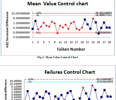
Fig-1: Mean Value Control Chart

Fig-2: Failure Control Chart

4. CONCLUSION

The failures control chart (Fig-1) and the mean value control chart (Fig-2) exemplifies that, the first out – of – control situation is noticed at the 10th failure with the corresponding successive difference of m(t) falling below the LCL. The two control charts using exponential and HLD shows the similar results Hence it is claimed that the failures control chart and mean value chart detects out - of - control in a positive way. Therefore, earlier detections are possible in failures control chart and mean value chart. Since both control mechanisms are making the detection at the same point, either mechanism based on Exponential Distribution [1] or Half Logistic Distribution [2] is preferable.

5. REFERENCES

Card D., (1994), Statistical Process Control for Software, IEEE Software, May, 95-97.

[1.] Card D., Berg R.A., (1989), An Industrial Engineering Approach to Software Development. J. Systems and Software, 10, 159-168.

[2.] Card D., Glass R.L., (1990), Measuring Software Design Quality, Prentice Hall

[3.] Cohen, A.C. and Whitten, B. (1980). Modified moment and maximum likelihood estimators for parameters of the three-parameter gamma distri-bution. Commun.Statist. -Simu. Comp. 11, 197{216. [4.] Ebenau R.G., (1994), Predictive Quality Control with

Software Inspections, Crosstalk, June.

[5.] Florac W.A., Carleton A.D., Bernard J.R., (2000), Statistical Process Control: Analyzing a Space Shuttle Onboard Software Process, IEEE Software,

[8.] Jalote P., (1999), CMM in Practice: Processes for Executing Software Projects at Infosys, Addison-Wesley.

[9.] K. Rosaiah, R. R. L. Kantam, G. Srinivasa Rao and P. Mallikharjuna Rao, ESTIMATION IN TRUNCATED

TYPE-I GENERALIZED LOGISTIC

DISTRIBUTION, Int. J. Agricult. Stat. Sci., Vol. 5, No. 2, pp. 317-325, 2009

[10.]M.Xie, T.N. Goh, P. Rajan; Some effective control chart procedures for reliability monitoring; Elsevier science Ltd, Reliability Engineering and system safety 77(2002) 143- 150

[11.]Mehrotra, K.G. and Nanda, P. (1974). Unbiased estimation of parameters by order Statistics in the case of censored samples. Biometrika, 61, 601{606. [12.]Mutsumi Komuro; Experiences of Applying SPC

Techniques to software development processes; 2006 ACM 1-59593-085-x/06/0005.

[13.]Paulk M.C., (2001), Applying SPC to the Personal Software Process, Proceedings of the 10th International. Conference on Software Quality, October

[14.]Persson, T and Rootzen, H. (1977). Simple highly efficient estimators for a Type I censored normal sample. Biometrika, 64, 123{128.

[15.]R Satya Prasad, Bandla Sreenivasa Rao, Dr. R.R. L Kantham, Monitoring Software Reliability using Statistical Process Control: An MMLE Approach, International Journal of Computer Science & Information Technology (IJCSIT) Vol 3, No 5, Oct 2011

[16.] R Satya Prasad, K Ramchand H Rao Rao, Dr. R.R. L Kantham, Software Reliability Measuring

UCL

33.35125694

CL

16.69817101

LCL

0.045085061

0.010000000

0.050000000

0.250000000

1.250000000

6.250000000

31.250000000

1

3

5

7 9 11 13 15 17 19 21 23 25 27 29

m

(t)

S

u

cc

es

iv

e

Di

ff

er

en

ce

Failure Number

Mean Value Control chart

UCL

31.23462967

CL

15.63842905

LCL

0.042223764

0.02000

0.04000

0.08000

0.16000

0.32000

0.64000

1.28000

2.56000

5.12000

10.24000

20.48000

1

3

5

7

9 11 13 15 17 19 21 23 25 27 29

m

(t

) s

u

cc

es

si

ve

d

if

fe

ren

ce

Failure Number

(5)

27 [18.]Tiku, M.L. (1988). Modified maximum

likelihood estimator for the bivariate normal. Commun. Statist.-Theor. Meth., 17, 893{910. [19.]Tiku, M.L. and Suresh, R.P. (1992). A new

method of estimation for location and scale parameters. J. Statist. Plann. & Inf. 30, 281-292, North- Holland.

[20.]Tiku, M.L., Wong, W. K., Vaughan, D.C. and Bian, G. (2000). Time series models in non-normal situations: symmetric innovations. Journal of Time Series Analysis, 21, 571{596.

[21.]Weller E., (1995), Applying Statistical Process Control to Software Maintenance. Proc. Applications of Software Measurement

[22.]Weller E., (2000), Applying Quantitative Methods to Software Maintenance, ASQ Software Quality Professional, 3 (1).