Munich Personal RePEc Archive
Calibrating Benefit Function Transfer to
Assess the Conservation Reserve
Program
Hellerstein, Daniel and Feather, Peter
Economic Research Service UDSA
1997
Online at
https://mpra.ub.uni-muenchen.de/25357/
Calibrating Benefit Function Transfer to Assess the Conservation Reserve Program
by
Peter Feather
and
Daniel Hellerstein*
*Environmental Economists at the U.S. Deptartment of Agriculture Economic Research
Calibrating Benefit Function Transfer
to Assess the Conservation Reserve Program
INTRODUCTION
Benefit transfer promises inexpensive measures of economic value in situations
of deficient data. In particular, benefit transfer allows for the generalization of a
narrowly focused study to a larger region, thereby avoiding potentially costly replications
of the original study. In response to legislative requirements that non-market benefits
be counted, and public sector budget constraints, the use of benefit transfer by
government agencies has intensified.
For example, the Damage Assessment Center at the National Oceanographic
and Atmospheric Administration (NOAA) assesses the damages resulting from small
"Type-A" spills or accidents using the National Resource Damage Assessment Model
for Coastal and Marine Environments (French et al., 1995).1 This model uses benefit
estimates from various sources to produce damage assessments based on limited
physical information from the spill site. Another application of benefit transfer is the
U.S. Forest Service's development of Resources Planning Act values for national
forests to use in long range planning processes to meet the requirements of the
National Forest Management Act.
1 For example, the Comprehensive Environmental Responses, Compensation and Liability Act
A crucial distinction in benefit transfer involves whether to transfer point
estimates (such as user day values) or the benefit function itself (such as the demand
function from which day use values are computed). Transferring point estimates from
the “study area” to the unstudied “policy area” is a common practice, especially in
federal government planning and procedures2. Benefit function transfer, in contrast,
involves use of the benefit function itself, in conjunction with demographic and
physical/biological data from the affected policy area. Since function transfer
recognizes the unique physical and demographic characteristics of the policy area, it is
argued (Loomis 1992) that estimates derived using function transfer are superior to
simpler, but undifferentiated, point transfer estimates.
The accuracy of benefit function transfer will depend on the degree of similarity
between the study area and the policy area. Large differences in the non-market
commodities, population demographics and social institutions will tend to create large
bias. The strength of benefit function transfer, as opposed to point estimate transfer, is
that we account for some of these differences. In practice, since all studies are
imperfect, and since exactly appropriate data may often be difficult to obtain, a potential
for bias exists. In consequence, methods of reducing such biases should be
considered..
The objective of this study is to develop national estimates of the non-market
water-based recreational benefits of reductions in soil erosion through the use of benefit
function transfer. The focus is on the water quality impacts of the Conservation
Reserve Program3 and other agricultural policies such as the adoption of BMPs (better
management practices). The first step involves estimating a recreational demand model
based on individual observations for four states from the 1992 National Survey of
Recreation and the Environment. Next, the functional form of the model is transferred
to the nation using county level U.S. Census data. This procedure incurs a risk of bias
due to the transfer of a function to a policy area for which only aggregate information is
available (e.g., Desvouges et al. 1992). Thus, a key element of the transfer
procedure is an explicit correction for possible aggregation bias.
.
CONDUCTING BENEFIT FUNCTION TRANSFER
Transferring a benefit function involves selecting a proper function to transfer,
gathering data to estimate benefits at the policy area, and calculating welfare changes
at the policy area using the transferred function. 4 The welfare function [W(P,D,Q)],
estimated at study area “s,” is a function of the prices (P), demographic characteristics
(D) and environmental quality (Q) of the inhabitants of the study area. In a given study
area s (say, a single county), total welfare (W1) might be estimated as the average
individual welfare of the i=1..Ns survey respondents times the county population (POPs),
which equals:
(1) W1s = POPs*{ΣiW(Pi,Di,Q )/Ns}. i = 1,...,Ns
Another estimator of welfare uses aggregate information, such as county
averages obtained from the U.S Census. Using such information, an aggregated
measure of total welfare in the county might be estimated as the welfare of the county
specific representative individual times the county population (POPs):
(2) W2s = POPs*W(E(Ps),E(Ds),Qs),
where E(Ps) and E(Ds) are the expected price and demographics of the representative
individual of county s.
Given that one’s sample is randomly drawn and therefore representative, W1s will
provide a consistent estimate of the population’s welfare. In contrast, for typically
non-linear welfare functions, W2s will not equal W1s, and furthermore W2s will be a
biased measure of the population welfare (Hellerstein, 1995).5 Therefore, when
transferring one’s results to policy area “t”, the use of W2t
(W2t=POPt*W(E(Pt),E(Dt),Qt)), is subject to bias. However, since individual data is
not likely to be available for area, W2 may be the only available option for measuring
welfare.
Examining the magnitude of this bias in the study area may provide information
that would be useful in calibrating W2t in the policy area. One possibility is to compute
W2s (in the study area) using aggregated data. Given a measure of W1s, estimates of
W2t in the policy area could be calibrated by the ratio W1s/W2s (from the study area).
A more ambitious approach, and the one used in this paper, involves computing a
location (county) specific "calibration function" (C) to be transferred along with the
benefit function.
The calibration function is computed using the original survey data, along with a
set of aggregate measures of distinct locations (say, counties) within the survey area.6
The following procedure is then used:
i) Compute W1s and W2s for each of the s=1..S distinct regions.
ii) Estimate γ in cs=C(Zs,γ), where cs=W1s/W2s and Zs is a set of aggregate
5 Jensen's inequality (see Mood et al.) states that if X is a random variable and f(•) is a concave
function, then E[f(X)] ≤ f(E[X]).
variables that may include E(Ps), E(Ds) and Qs.
iii) Compute ct=C(Zt,γ).
iv) Compute a calibrated welfare measure for the policy area as the product W2t
x ct.
sample.
The choice of the Z variables will depend on data availability. Since the deviation of W2
from W1 will worsen as intra-location variation increases, inclusion of measues of the
variance of the explanatory variables, as well as their averages, is advisable.
Examples of this would include the standard deviation of income, along with per capita
income.
THE DATA
Recreational trip taking information comes from the 1992 National Survey of
Recreation and the Environment (NSRE), a large survey aimed at providing national
data for several recreational activities. One component of the NSRE is a survey of
water based recreational activities in four "area study" regions in the U.S.7 This study
is based on these results.8 Respondents were asked to recall the number of trips taken
to up three wetlands, three lakes and three rivers that were less than 100 miles from
their residence within the last 12 months where the presence of water was an important
reason for taking the trip. The name of each destination as well as its distance and
direction (e.g., north, north east, east, etc.) from the respondent's residence were
obtained. When possible, destination names were matched to area maps to recover
the location (latitude and longitude) of each destination. If the map location could not
be determined, then the self reported distance and direction was used to determine the
location of the trip destination.
7 These four "area study regions" are located in Indiana, Nebraska, Pennsylvania and Washington.
The resulting data contains information about the water based recreation of
about 1500 persons evenly divided among the four area study regions. About 50% of
the respondents participated in any water based activity with an average annual
participation rate of approximately 16 trips over the year. To capture the intrinsic
differences between lake and river based recreation, lake and river trips are modelled
separately9.
The physical conditions at the destinations themselves are described by data
from the 1992 National Resources Inventory (NRI). The 1992 NRI is the most recent of
a series of inventories conducted every five years by the U.S. Department of
Agriculture's Natural Resources Conservation Service (NRCS)10. It contains information
on the status, condition, and trends of land, soil, water and related resources on
non-Federal land in the U.S.11 The survey is scientifically designed and based on
recognized statistical sampling methods. Data are collected for the 1992 NRI for more
than 800,000 locations (points) by NRCS personnel. Each datum, or point, represents
a homogenous area of land of varying size. Although the geographic location of each
point is known, it is not available to preserve the anonymity of the land owner. To use
the data in a geographic analysis, White et. al. (1989) has suggested the formation of
"NRI polygons" based on the NRI sample point identifier. Each sample point carries an
identifier placing it in one of 3,041 counties, 209 Major Land Resource Areas and 2,111
hydrological units. Intersecting these boundaries results in 14,414 NRI polygons for the
48 conterminous states in the U.S. that contain at least one NRI point. The average
polygon size is 102,518 acres, ranging from a minimum of 1,290 acres to a maximum of
677,647 acres. The point specific information in each polygon can be aggregated to a
polygon level observation using an area weighted average. The average attribute for
the j-th polygon (Aj) is represented by:
(3) Aj = (Σi∈jAi * Areai)(Σi∈jAreai),
10 Formerly known as the Soil Conservation Service.
where i indexes NRI points in polygon j, Areai is the area of the i-th NRI point and Ai is
the attribute of the i-th NRI point.
Since confidentiality restrictions preclude the use of of point specific information,
these aggregate polygon are used to define trip sites. Instead of specifying individual
lake and river locations as destinations, the locations were mapped into NRI polygons.
Five variables describe each destination (NRI polygon)12. Trip cost is the travel cost
from the centroid of the respondent's zip code zone to the centroid of the NRI polygon13.
Two variables indicating land characteristics in the polygon are the percentage forested
area and percentage privately owned area. A priori, the expectation is that large
amounts of privately owned land represent a lack of recreational opportunities while
large amounts of forested land augment recreational quality. Average erosion in each
polygon is the average sheet and rill soil erosion in tons/acre calculated using the
universal soil loss equation (USLE)14. This variable is used as an indicator of water
quality at each destination. Changes in erosion are assumed to produce changes in
water quality, which then impacts the enjoyment of recreational activities.
Is There a Relationship Between Erosion and Water Quality?
12 To be consistent with the survey questions, any polygons further than 100 miles of the respondent's residence were not assumed to be in the choice set of trip destinations.
13 Trip cost is the round trip travel cost (distance*$0.35) plus the round trip time cost ((personal
income)*0.333*distance/50).
The early stages of this analysis included the collection of biological water quality
data from the EPA Storet system for the years 1990-1994 in the four area study states.
The goal was to construct a physical model capable of predicting changes in water
quality resulting from changes in erosion. The resulting data are too limited to produce
a reliable physical model, but do provide some evidence of a relationship between water
quality measures (total nitrates, total phosphorous and dissolved oxygen) and erosion
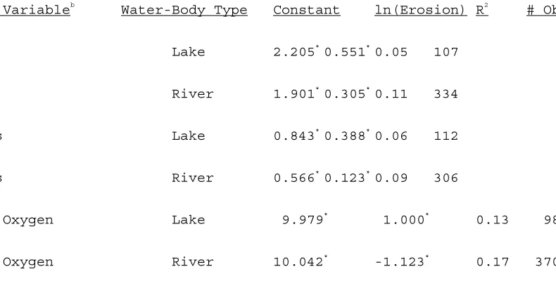
levels. To investigate this relationship, average water quality variables15 for lakes and
rivers were regressed on a constant term and the natural logarithm of the polygon
erosion rate. All of the regression parameters (Table 1) are of the anticipated positive
sign except for the dissolved oxygen model for rivers. The low R2 statistics associated
with all six models may be the result of removing variation from the water quality data by
averaging it over sampling points and polygons. It is also a likely indication that water
quality is affected by many factors other than erosion. Despite the low R2 statistics, the
sign and significance of most of the erosion parameters lend some support to a
relationship between water quality and ambient erosion.
THE MODEL
The benefit function is estimated using a two stage discrete-count demand model
similar to that proposed by Feather et al. (1995). The first stage is a random utility
model (RUM) describing the choice of destination on a recreational outing. The
strength of the RUM is that it captures substitution among competing sites when quality
changes occur. The drawback of the RUM is its inability to account for changes in the
total quantity of trips when changes in site quality occur. Both of these questions are
important because quality changes presumably create two effects: substitution amongst
sites and changes in participation. To better address the participation component of
the problem, a secondary participation model is often estimated. These models allow
for changes in participation to occur when changes in site quality occur. Both
components of this model are described below along with estimation results.
The RUM is commonly used to estimate situations referred to as "corner solutions" where one, or a few goods are chosen from a larger set of substitutable goods. This large choice set is composed of all relevant "elemental alternatives" [Ben-Akiva and Lerman (1985)]. For example, all lakes within a few hours drive from an individual's home may form the set of elemental alternatives for a certain type of water based recreation. The random utility of elemental alternative l to individual k [Ulk]
is written as:
(4) Ulk = Vlk + εlk, l = 1,...,L k = 1,...,N
where Vlk is the deterministic portion of the utility function and εlk is an independently
and identically distributed extreme value random variable with mode 0 and scale
parameter μ. Typically, Vlk is written as a linear function of income (Yk), the cost
incurred in visiting the site (Clk), and a vector of characteristics describing the site
(bl=[bl1,...,blm]):
(5) Vlk = β(Yk-Clk) + Θbl,
where β and Θ = [Θ1,...,Θm] are parameters to be estimated. It is well known that the
parameters of Vlk can be estimated using a multinomial logit model:
where Pk(l) is the probability of individual k choosing elemental alternative l.
The use of aggregated alternatives (i.e., NRI polygons) adds bias to the RUM
which can be partially removed by including a measure of size in the indirect utility
function. Denote the i-th aggregated alternative (polygon) as Li where Li is a mutually
exclusive set of elemental alternatives. The random utility of the k-th individual
choosing an elemental alternative contained in the set Li [Uik] is:
(7) Uik = Max(Vlk + εlk) ∀ l ∈ Li
It has been shown [see Parsons and Needelman (1992)] that (7) can be decomposed
into:
(8) Uik = V*ik + (1/μ)ln(Mi) + (1/μ)ln(Bi) + εik,
where V*ik is the average utility of the i-th aggregate alternative, Mi is the number of
elemental alternatives in the i-th aggregate alternative, and Bi is a measure of the
variability of the utilities of the elemental alternatives in the i-th aggregate alternative:
(9) Bi = Σlexp[μ(Vlk - V*ik)]/Mi, ∀ l ∈ Li.
Since Bi depends on Vlk, it cannot be recovered. Operationally, the aggregate model is
estimated as:
(10) Pk(i) = exp{V*ik+(1/μ)ln(Mi)}/Σjexp{V*jk+(1/μ)ln(Mj)},
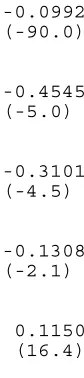
Estimation results of this portion of the model appear in Table 2. Although the
signs of the parameters in each model are identical, parameter magnitudes and levels
of significance vary. In each model, trip cost is significant and negative indicating that
respondents prefer closer locations to further ones. The parameters associated with
unexpectedly negative. This may indicate that heavily forested areas are less
accessible to recreationalists. The parameters associated with the percentage of
privately owned land, which is assumed to represent a lack of recreational opportunities,
are negative as anticipated. Average erosion has an anticipated negative sign in both
models suggesting that more water based recreation occurs in areas with low erosion
rates. The final variable, Log(Size), is the correction factor for aggregation bias (Mi)16.
The RUM addresses the decision of where to go, but ignores the decision of
"how much to go". Changes in destination qualities cause visitation probabilities to
change allowing for substitution amongst destinations. Changes in total participation
and decisions of whether or not to participate at all cannot be accounted for using this
first stage of the model. Several options exist for linking the RUM model to a
continuous model that incorporates participation decisions (see for example Bockstael
et al., 1987; Morey et al., 1993; Parsons and Kealy, 1995; Feather et al. 1995). Most
advocate using information from the RUM, and socio-economic variables in a
"participation equation". This study uses a method proposed by Feather et al. (1995).
The approach consists of estimating total participation, (Tk), as a function of expected
trip costs, E(Ck), expected destination qualities, E(bk), Income, Yk, and socio economic
variables, S:
(11) Tk = fk(E(Ck),E(bk),Yk,S).
Expected costs and qualities are calculated from the first stage RUM:
(12) E(Ck)=ΣiPk(i)Cik,
(13) E(bk)=ΣiPk(i)bi,
where k indexes individuals and i indexes aggregate alternatives. Participation is assumed to be directly related to expected quality and inversely related to expected costs. Changes in destination quality will change destination probabilities in (10) which will change expected costs and qualities in (12) and (13). Treating (11) as a demand equation allows for conventional welfare measures resulting from quality changes to be computed. Changes in expected costs cause movements along the demand function while changes in expected qualities cause shifts in the demand function. The resulting change in welfare (ΔW) is the difference in consumer surplus between the final cost and quality state (Ck1,bk1) and the initial cost and quality state (Ck0,bk0):
⌠∞ ⌠∞
(14) ΔW = ⎮ fk1(E(Ck1),E(bk1),Yk,S)dCk - ⎮fk0(E(Ck0),E(bk0),Yk,S)dCk.
⌡Ck1 ⌡Ck0
To accommodate decisions of zero and nonzero participation, (11) is estimated
using a double hurdle count model (see Yen, 1993; Blisard and Blaylock, 1993;
Shonkwiler, 1994). Essentially, this model assumes that two "hurdles", or different sets
of variables, determine consumption. The first (Zk) depends on mainly demographic
variables (age, gender, education, etc.) while the second (Xk) depends mainly on
economic variables (price, quality, etc.). Let Dk denote the latent decision to participate
where participation (Tk) equals zero if Dk≤ 0:
(15) E(Dk) = Γk = exp(Zk'τ).
When observed participation is positive (Tk > 0), then observed participation equals
desired participation (Tk*) where:
(16) E(Tk*) = λk = exp(Pkδ+Xk'α),
are parameters to be estimated. In the double hurdle poisson model, the probability of
observing zero participation is:
(17) Pr(Tk = 0) = Pr(Tk*≤ 0) + Pr(Tk* > 0)Pr(Dk≤ 0)
= exp(-λk)+(1-exp(-λk))exp(-Γk).
The probability of observing positive participation is:
(18) Pr(Tk > 0) = Pr(Tk* > 0)Pr(Tk*|Tk* > 0)Pr(Dk > 0)
= (1-exp(Γk))exp(-λk)λTk/Tk!.
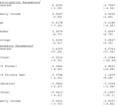
Expected trip cost and quality, along with income, describe the intensity of
participation (Xk) variables in the double hurdle model. The variables affecting the
decision to participate (Zk) are income, age, gender and education. The estimation
results in Table 3 show that both sets of variables are generally significant and
consistent in sign across the lake and river recreation models. Higher incomes and
levels of education are positively associated with participation while age is negatively
associated with participation. A gender dummy variable suggests that males tend to be
participants more often than females. The second stage variables represent the
decision of how much to participate and are anticipated to have the same sign as those
in the RUM. This is generally true with the exception of % Forest and % Private Own in
the river model and the expected size variable in both models. Income, which is
assumed to effect both the intensity and the participation, is negative indicating that avid
participants tend to have lower income levels.
In the double hurdle poisson model, expected consumer surplus for the k-th
individual is (E(CSk)):
Welfare changes (ΔW) are the difference in expected consumer surplus from the final
state, E(CSk''), to the initial state, E(CSk'),:
(20) ΔW = E(CSk'') - E(CSk').
TRANSFER AND WELFARE RESULTS
Transferring the model to the nation requires a national data set of environmental
quality and demographic information. National environmental quality information is
provided by the NRI. National demographic information is provided by the U.S.
Census. A "representative individual" was constructed in each of the 3,071 counties in
the 48 conterminous states using the 1990 U.S. Census. By assumption, this individual
resides in the geographic centroid of the county, has the average income, age, gender
and education found in the county, and faces a recreational choice set of NRI polygons
within 100 miles of the county centroid.
Three hypothetical changes in erosion are considered based on 1982 NRI
erosion levels17. 1982 levels are used because they reflect erosion rates that prevailed
before the effect of the Conservation Reserve Program (CRP), initiated i 1985, was
observed. All three scenarios represent an increase in the current average erosion
rate of 1.283 tons per acre:
Scenario #1: Change erosion rates to the 1982 level for all agricultural and
non-agricultural land. This is the national erosion level in 1982 which was 1.681 tons per acre on average.
Scenario #2: Change erosion to the 1982 level for land that were either cropland in 1992, or cropland in 1982. Leave all other land at the 1992 level.
This is the change in erosion that occurred on agricultural land over the past decade. The average erosion rate under this scenario is 1.654 tons per acre.
Scenario #3: Change erosion to 1982 level on all land that is currently enrolled in the
CRP, leave all other areas at the 1992 level. This is the change in
erosion attributable to the CRP. The average erosion rate under
this scenario is 1.289 tons per acre.
Before transferring the benefit function to the nation as a whole, welfare
measures were computed in the study area using the NSRE data and the Census
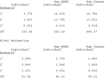
data. Table 4 shows changes in welfare and total consumer surplus computed using
three aggregation approaches. The first column contains the average welfare
measures computed using the individual NSRE data. This is the approximate "true"
measure in (1) before being multiplied by population. The third column contains
averages using representative individual data from the U.S. Census. This is the
measure in (2) that will be computed in the policy area before being multiplied by
population. The large differences between column one and three suggest that
significant bias may occur when the function is transferred. The bias comes both from
nonlinearity in the benefit function and disparities between the NSRE data and the
Census data. The second column in Table 4 helps to separate the effects. This
column contains average welfare measures computed by creating representative county
individuals from the NSRE data. Since the welfare measures in columns one and two
are based on the same data, differences between these columns result from the
nonlinearity of the benefit function. Differences between columns two and three result
4 suggest that nonlinearity in the benefit function causes a large portion of the bias that
occurs in the transfer.
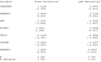
To account for the transfer bias, a "calibration function" is estimated using these
welfare estimates. This involves regressing the ratio of county average individual
consumer surplus (column one in Table 4) to county representative consumer surplus
(column three in Table 4) on county Census information18. Estimation results appear in
Table 5. Demographic variables appearing in the benefit function, as well as proxies of
their variances are used to predict the ratio described above. Measures of age (AGE),
proportion of elderly in the county (AGEGE65) and low income households in the county
(INC20) explain most of the variation in the welfare ratio.
18 Price and quality information is not included in the estimation because these data do not change when the benefit function is transferred.
The welfare experiments consist of first calculating a hypothetical erosion rate for
each NRI polygon. Next, expected costs and qualities are calculated under both the
observed (1992) erosion rate and the hypothetical erosion rate using (12) and (13).
These expected variables, along with the demographic county specific information, are
used in (20) to compute a welfare measure for each representative individual. The
individual's welfare measure is then aggregated to the county level by multiplying it by
the county population and the predicted calibration ratio. The individual county
measures are then summed to arrive at a national estimate of the change in welfare due
to the hypothetical change in erosion.
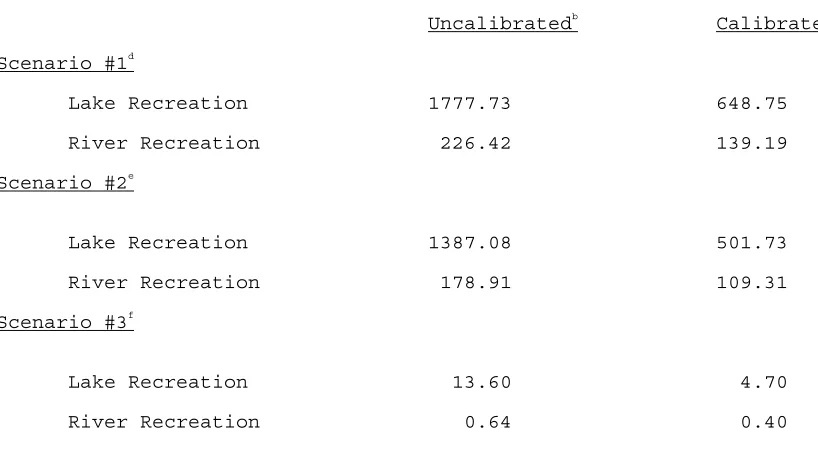
Both calibrated and uncalibrated welfare estimates appear in Table 6. The
benefit estimates are less than half of the uncalibrated estimates for lake recreation and
two thirds of the uncalibrated estimates for river recreation. The following discussion
relies on the calibrated welfare measures since they are an estimate of the "true"
welfare in (1).
The welfare estimates show that lake users are impacted by each of the
scenarios much more than river users. The likely reason for this is the more intensive
use of lakes as opposed to rivers for water quality sensitive contact types of activities.
The estimates also show that most of the benefits of erosion reduction occurring from
1982 to 1992 are attributable to better management of agricultural lands. Comparing
scenario #1 to scenario #2 shows the portion of benefits attributed to changes in erosion
on agricultural lands. Approximately 78% ($611.04 million) of the $787.94 million in
annual benefits and 98% of the total erosion reductions over the previous 10 years can
be attributed to erosion control on agricultural lands. The third scenario measuring the
effect of the CRP shows that the water based recreational benefits associated with this
program are relatively small. Less than 1%, or $5.1 million, of the benefits attributed to
agricultural erosion control are a result of the CRP. This is because the reduction in
erosion attributable to the CRP is small19. Approximately 60% of the 35.4 million acres
of CRP land has high wind erosion rates, and negligible sheet and rill (soil) erosion
(Osborn, et. al (1992)). Changes is erosion on this land does not contribute toward any
recreational benefits because the analysis assumes that wind erosion has no impact on
water quality.
Few studies exist to compare these results to. Clark et. al (1981) estimated
cropland's annual contribution to erosion based damage to all water based recreational
damages to be $1.24 billion (adjusted to 1994 dollars). This number reflects the
benefits that would occur if the detrimental effects of erosion on water quality from
agricultural lands were eliminated. A more recent study by Ribaudo (1989) places the
annual benefits of the CRP to freshwater fishing at $69.7 million (adjusted to 1994
dollars). Ribaudo estimated a physical model relating sediment discharges, stream
flow and water storage to pollutant concentrations in aggregated sub-areas of the U.S.
He then predicted the CRP's effect on pollutant concentrations (via sediment
discharges) and used this information in a trip day intensity prediction model. Changes
in days of participation were multiplied by an independent per fishing day value ($25.00)
to arrive at the welfare estimate. Although Ribaudo's work benefits from using a
physical model relating erosion with pollutant levels, it has the drawback of using much
more aggregated destinations than were used in this study and relying on transferring a
point estimate instead of a benefit function to determine welfare measures.
SUMMARY AND CONCLUSIONS
Refining methods of benefit transfer techniques is essential due to its increasing
use in policy analysis. Benefit transfer offers a reliable short cut to an expensive and
time consuming original analysis only if it is carefully applied. Although benefit function
transfer is recognized to be superior to simply transferring a point estimate, the
recognizing and dealing with the bias resulting from deriving benefits for representative
individuals from benefit functions estimated using individual observations. Due to
nonlinearities in the benefit function, the transferred function may provide a poor
estimate of the welfare change at the policy site.
In this study, a model used to evaluate the recreational benefits of soil erosion
reductions that occurred over the past decade on agricultural lands is estimated in four
study areas and transferred nationwide. Comparing welfare measures computed using
individual observations versus representative data in the study area indicated that large
biases will result when the transfer is performed due to nonlinearities in the benefit
function. To adjust for this, information from the study area in the form of a calibration
function was transferred along with the benefit function. This allowed the national
benefit estimates to be adjusted for the effect of using representative data to estimate
national welfare measures.
The national benefit measures themselves indicate that erosion reductions on
agricultural lands over the past decade have generated large recreational benefits.
National reductions in erosion are estimated to be $787.94 million with $611.04 million
being attributed to agricultural erosion reductions. The benefits attributed to the CRP
are less than 1% ($5.1 million) of the agricultural benefits. This relatively small share of
CRP benefits occurs because over half of the CRP is on lands with high levels of wind
erosion, not sheet and rill (soil) erosion. The analysis assumes that wind erosion has
no effect on water quality. The remaining CRP acreage is small compared to the total
amount of agricultural land in the nation. Thus, changes in erosion on this land has a
This, as with most national studies, is not without faults. The analysis is based
on four regional samples of water based recreation that are assumed to be
representative of the nation as a whole. Erosion rates, instead of actual water quality
variables, are assumed to influence behavior. Additionally, "sites" are defined as
aggregate NRI polygons instead of individual lakes and streams. As discussed in the
data section, there is some evidence that water quality measures are statistically
influenced by erosion. Whether these measures influence recreational behavior is
unknown. The bias associated with using aggregated sites is somewhat, but not
completely, removed by including a size measure in the RUM specification. While the
issue of the four regional samples being representative of the behavior of individuals
nation-wide cannot be addressed, more data would increase the accuracy of the
References
Ben-Akiva, M. and S. Lerman. Discrete Choice Analysis: Theory and Application to Travel Demand. 1985 Cambridge: The MIT Press.
Blisard, N and J. Blaylock. "Distinguishing Between Market Participation and Infrequency of Purchase Models of Butter Demand." American Journal of Agricultural Economics. 75(May 1993): 314-320.
Bockstael, N., W. Hanemann, and C. Kling. "Estimating the Value of Water Quality Improvements in a Recreational Demand Framework." Water Resources Research. 23(May 1987): 951-960.
Boyle, K. and J. Bergstrom. "Benefit Transfer Studies: Myths, Pragmatism, and Idealism." Water Resources Research, Vol. 28, No. 3, March 1992, pp. 657-663.
Clark, E. , J Haverkampn and W. Chapman. Eroding Soils: The Off-Farm Impacts. Washington, DC: The Conservation Foundation, 1985.
Desvousges, W., M. Naughton, and G. Parsons. "Benefit Transfer: Conceptual Problems in Estimating Water Quality Benefits Using Existing Studies." Water Resources Research, Vol. 28, No. 3, March 1992, pp. 675-683.
Feather, P., D. Hellerstein, and T. Tomasi. "A Discrete-Count Model of
Recreational Demand." Journal of Environmental Economics and Management.
29(September 1993): 214-227.
Hay, M. "Net Economic Recreational Values for Deer, Elk and Waterfowl Hunting and Bass Fishing." U.S. Department of the Interior, Fish and Wildlife Service, Report 85-1, July, 1988a.
Hay, M. "Net Economic Values of Nonconsumptive Wildlife-Related Recreation." U.S. Department of the Interior, Fish and Wildlife Service, Report 85-2, August, 1988b.
Hellerstein, Daniel. “Welfare Estimation Using Aggregate and
Henderson, J. "Corps. of Engineers Regional Recreational Demand Model." Paper presented at W-133 Regional project Meeting, Monterey, CA, February, 1991.
Loomis, J. "The Evolution of a More Rigorous Approach to Benefit Transfer: Benefit Function Transfer." Water Resources Research, Vol. 28, No. 3, March 1992, pp. 701-705.
Luken, R., F. Johnson and V. Kibler. "Benefits and Costs of Pulp and Paper Effluent Controls Under the Clean Water Act." Water Resources Research, Vol. 28, No. 3, March 1992, pp. 665-674.
McConnell, K. "Model Building and Judgement: Implications for Benefit
Transfers and Travel Cost Models." Water Resources Research, Vol. 28, No. 3, March 1992, pp. 695-700.
Mood, A., F. Graybill and D. Boes. Introduction to the Theory of Statistics. New York, McGraw-Hill Book Company, 1963.
Morey, E., D. Rowe, and M. Watson. "A Repeated Nested-Logit Model of Atlantic Salmon Fishing." American Journal of Agricultural Economics. 75(August 1993): 578-592.
Osborn. C. T., F. Llacuna, and M. Linsenbigler. The Conservation Reserve Program: Enrollment Statistics for Signup Periods 1-11 and Fiscal Years 1990-1992. USDA-ERS-SBN #843(November 1992).
Parsons, G., and M. Kealy. "A Demand Theory for Number of Trips in a Random Utility Model of Recreation." Journal of Environmental Economics and Management. (Forthcoming: December 1995).
Parsons, G., and M. Needelman. "Site Aggregation in a Random Utility Model of Recreation." Land Economics. 68(November 1992): 418-433.
Ribaudo, M. Water Quality Benefits From the Conservation Reserve Program. USDA-ERS AER #606 (February 1989).
Shonkwiler, J. "Double Hurdle Count Data Models for Travel Cost Analysis." Unpublished paper presented at the W-133 Meetings, Tucson, AZ. Feb 23-25, 1994.
White, D., M. Maizel, K. Chan, and J. Corson-Rikert. "Polygon Overlay to Support Point Sample Mapping: The National Resources Inventory." Auto-Carto TX, Baltimore, MD, pp. 33-37. 1989.
Waddington, D., K. Boyle and J. Cooper. "1991 Net Economic Values for Bass and Trout Fishing, Deer Hunting, and Wildlife Watching." U.S. Department of the Interior, Fish and Wildlife Service, Report 91-1, October, 1994.
Table 1 - Linear Regression of Water Quality Measures on 1992 Soil Erosiona
Dependent Variableb
Water-Body Type Constant ln(Erosion) R2
# Obs
Nitrates Lake 2.205*
0.551*
0.05 107
Nitrates River 1.901*
0.305*
0.11 334
Phosphates Lake 0.843*
0.388*
0.06 112
Phosphates River 0.566* 0.123* 0.09 306
Dissolved Oxygen Lake 9.979*
1.000*
0.13 98
Dissolved Oxygen River 10.042*
-1.123*
0.17 370
a
Water quality data (Dependent Variable) from EPA STORET system is averaged over a unique location then over the NRI polygon by type of water body. Average water quality is then regressed on average weighted NRI polygon erosion (tons/acre) calculated using the USLE.
b
Nitrates are total dissolved nitrates in mg/l; Phosphates are total phosphates in mg/l; Dissolved Oxygen is total dissolved oxygen in mg/l
Table 2 -- Random Utility Models of Lake and River Recreationa
Lake Recreation Modelb
River Recreation Modelc
Parametersd
Trip Cost -0.0834 -0.0992
(-108.1) (-90.0)
% Forest -1.4271 -0.4545
(-18.4) (-5.0)
% Privately Owned -1.0778 -0.3101
(-19.3) (-4.5)
Erosion -0.1511 -0.1308
(-18.1) (-2.1)
Log(Size) 0.0141 0.1150
(5.5) (16.4)
a
Random utility models based on water oriented recreational activities at lakes and rivers. t-statistics for the null hypothesis that the parameter equals zero appear in parenthesis.
b
Estimated using a sample of 706 individuals averaging 9.78 lake based trips per person. Most participants visited more than one location over the year; the number of unique respondent/location pairs is 1323.
c
Estimated using a sample of 447 individuals averaging 10.81 river based trips per person. Most participants visited more than one location over the year; the number of unique respondent/location pairs is 772.
d
Table 3 -- Double Hurdle Poisson Models of Lake and River Based Recreationa
Lake Recreation Modelb
River Recreation Modelc
Participation Parametersd
Constant -0.2183 -0.7567
(-1.59) (-4.36)
Family Income 0.0067 0.0035
(3.59) (1.49)
Age -0.0178 -0.0186
(-7.30) (-6.05)
Gender 0.3679 0.6567
(4.71) (6.79)
College 0.2191 0.0827
(2.51) (0.76)
Intensity Parameterse
Constant 3.6353 6.2761
(37.28) (37.09)
E(Cost) -0.0214 -0.1044
(-5.30) (-20.65)
E(% Forest) -0.3466 0.8621
(-4.59) (12.98)
E(% Private Own) -0.3784 1.1479
(-2.53) (8.29)
E(Erosion) -0.0462 -0.0309
(-2.47) (-2.99)
E(Size) -0.0413 -0.1927
(-4.21) (-16.1)
Family Income -0.0021 -0.0057
(-3.70) (-9.85)
a
Double Hurdle Poisson models of lake and river based recreation participation and intensity.
b
Estimated using a sample of 1510 survey respondents consisting of 706 participants and 804 nonparticipants.
c
Estimated using a sample of 1510 survey respondents consisting of 447 participants and 1063 nonparticipants.
d
Constant is a constant term. Family Income is the respondent's family income in dollars. Age is the respondent's age in years. Gender equals one if the respondent is male, zero otherwise. College equals one if the respondent has completed a college education.
e
Table 4 -- Comparison of Individual Welfare Levels in the Study Area
Lake Recreation
Rep NSRE Rep Census
Individuala Individualb Individualc
Scenariod
1e
3.776 14.635 14.782
2f
3.463 13.795 13.913
3g
0.001 0.015 0.018
CSh
232.46 663.22 684.37
River Recreation
Rep NSRE Rep Census
Individuala Individualb Individualc
Scenariod
1e
0.995 1.730 1.860
2f
0.866 1.546 1.660
3g
0.001 0.002 0.002
CSh
51.58 86.31 93.21
a
Change in welfare in $1.00 units is computed for each NSRE respondent then averaged over respondents. Results of averaging individuals within a county and then over counties made little difference.
b
Change in welfare is computed by creating a representative county resident from the NSRE data. This individual is assumed to reside in the county centroid. The resulting per county estimates were then averaged over all counties in the survey.
c
Change in welfare computed using representative individual data from the U.S. Census. The counties included are the same as those in the NSRE sample.
d
Change in welfare is initial consumer surplus (evaluated at 1992 erosion rate) minus final (scenario level) erosion rate. Scenario #1 changes erosion to 1982 level for all NRI points. Scenario #2 is change erosion to 1982 level for all NRI points except those that were not
cropland in 1982 and 1992 (these are left at the 1992 level).
g
Change erosion to 1982 level on all NRI points that are currently enrolled in the CRP, leave all other NRI points at the 1992 level.
h
Table 5 -- Calibration Function Estimatesa
Variableb
River Recreationc
Lake Recreationd
CONSTANT 1.2144 0.4970
(1.376) (1.633)
PERMALE 0.9956 0.3104
(0.625) (0.565)
AGE -0.0361 -0.0081
(-2.849) (-1.863)
HIGHSC 0.3041 0.0588
(1.084) (0.607)
INC20 -2.1149 -0.5982
(-2.766) (-2.268)
INCOME -0.0050 -0.0007
(-0.592) (-0.235)
AGEGE65 3.2893 0.5452
(2.935) (1.410)
R2
0.229 0.232
R2
-Adjusted 0.189 0.193
a
Least squares regression of observed county calibration factors on county data from the U.S. Census. Calibration factor is the average consumer surplus in each county from individual NSRE data divided by the consumer surplus of the
representative individual from the U.S. census. Sample size is 126.
b
Constant is the constant term; PERMALE is the proportion of the county that is male; AGE is the average age of persons in the county in years; HIGHSC is the proportion of persons in the county who have graduated from high school; INC1020 in the proportion of households in the county who have incomes less than $20,000 per year; INCOME is the median annual household income in the county in $1000.00 dollar units; AGEGE65 is the proportion of persons in the county who are 65 years
old or older. R2 (R2-Adjusted) is the (adjusted) coefficient of determination.
t-statistics for the null hypothesis that the parameter equals zero are in parenthesis. Sample size is 126.
c
For the river recreation model.
d
Table 6 -- National Welfare Calculationsa
Uncalibratedb
Calibratedc
Scenario #1d
Lake Recreation 1777.73 648.75
River Recreation 226.42 139.19
Scenario #2e
Lake Recreation 1387.08 501.73
River Recreation 178.91 109.31
Scenario #3f
Lake Recreation 13.60 4.70
River Recreation 0.64 0.40
a
Sum of change in expected consumer surplus (initial minus final) in million dollar units times county population for three scenarios of erosion changes. Initial quality state is 1992 USLE erosion rate in tons/acre.
b
Difference ($ million) in expected consumer surplus for representative county individual times county population.
c
Difference ($ million) in calibrated expected consumer surplus for representative county individual times county population.
d
Change erosion to 1982 level for all NRI points.
e
Change erosion to 1982 level for all NRI points except those that were not cropland in 1982 and 1992 (these are left at the 1992 level).
f