Theoretical and Numerical Analysis of Electrocatalytic Processes at Conducting Polymer Modified Electrodes

(1)

Theoretical and Numerical Analysis of Electro catalytic

Processes at Conducting Polymer Modified Electrodes

S.P. Ananthi

Govt. Boys Higher Secondary School, Thirumangalam, Madurai Tamilnadu, India

A. Meena, L.Rajendran

Department of Maths

The Madura College Madurai-625011 Tamilnadu, India

N. Ramaraj

G. K. M, College Dept. of Maths of The Madura

Engineering, College Chennai – 600063 Tamilnadu,

India

ABSTRACT

A theoretical model of an electrocatalytic processes taking place at conducting polymer modified electrodes is discussed. In this model the diffusion of solution species, charge carriers and chemical reaction within the film are taken into account. The model involves the system of non-linear non-steady-state reaction diffusion equations. Analytical expressions pertaining to the concentrations are obtained in terms of second-order reaction rate constant. Also simple theoretical expression of transient current is derived. In this paper, a powerful analytical method, called Homotopy analysis method (HAM) is used to obtain approximate solutions for a non-linear partial differential equation. The obtained approximate solution in comparison with the numerical ones is found to be in satisfactory agreement.

Keywords

Electrocatalysis; Polymer modified electrode; Polyaniline; Non-linear differential equations; Homotopy analysis method; Simulation;

1. INTRODUCTION

Non-linear phenomena play a crucial role in applied chemistry and physics. Problems of coupled diffusion and non-linear chemical reaction are often in practical situations. In such systems the diffusion of the chemical species into a phase is accompanied by chemical reaction either with species already present in the phase, or catalysed by species within the phase. Examples include the diffusion and reaction in immobilized enzyme membranes, diffusion into living cells and micro-organisms and chemical reactions in conducting polymers. Polymer-modified electrodes are particularly attractive for chemical sensing applications [1-7]. The operation of a polymer sensor operating under amperometric conditions is simple in concept: the redox-active substrate of interest reacts with active receptor sites immobilized within the polymer film matrix rather than at the underlying support electrode. Electrocatalysis at electrodes, covered with conducting polymers and related materials, presents a remarkable phenomenon that finds diverse applications, especially in sensors and biosensors [8, 9]. It is essential that, within the frame of this model, the chemical redox interaction of reactant with active centers within the polymer film has been supposed to proceed as a simple second-order chemical reaction. The conducting polymers in electrocatalytic systems have the following four simple process [10] . (i) The diffusion of reactant from solution into conducting polymer film (ii) A chemical reaction between the diffusing species and catalytically active centers within the polymer film. (iii) The diffusion of charge carriers from the electrode surface to reaction zone through polymer layer. (iv) The diffusion of reaction products out of a polymer layer into the bulk of solution.

Earlier Ivanauskas et al. [10, 11] presented a model of electrocatalytic processes at conducting polymer modified electrodes. Ivanauskas and co-workers obtained the concentration of reactant, reaction product and charge carrier, using the finite difference technique [10, 11]. To our knowledge, no general theoretical expressions for the concentrations and current have been reported for all values of the rate constant

k

. The purpose of this paper is to derive an analytical expression for the concentrations of chemical species and current for all values of the rate constant

k

and time t using Homotopy analysis method (HAM).

2. MATHEMATICAL FORMULATION

OF THE PROBLEM

Building upon earlier works, Ivanauskas et. al [10] presented a concise assumption, discussion and derivation of the mass transport equations for this model which is summarized briefly below. In modeling of electrocatalysis at conducting polymer coated electrode [11], it is assumed that a flat surface of electrode is covered with a uniform layer of a conducting polymer of a definite thickness d. The schematic representation of the polymer modified electrode is given in Fig. 1.

The electrochemical charge transfer process was performed assuming the following reduction scheme [ 11 ]:

P

n

R

k





₍₁₎

where R and P are reactant and reaction product, respectively, and n is a charge carrier, i.e., an electron for cathodic reduction, or for anodic oxidation processes and k is a second-order rate constant for the chemical reaction. The non-steady-state reaction-diffusion equations governing the transport of electroactive species for the reaction scheme (1) are as follows [11]:

 

_{   }

t

x

n

t

x

kR

x

t

x

R

D

t

x

R

,

2









(2)

 

_{   }

t

x

n

t

x

kR

x

t

x

P

D

t

x

P

,

2









(3)

 

_{   }

t

x

n

t

x

kR

x

t

x

n

D

t

x

n

,

2









(4) where

x

and

t

stand for space and time, respectively.

)

,

(

x

t

R

_,

P

(

x

,

t

)

_and

n

(

x

,

t

)

_{denote the concentrations}

of the reactant, product and charge carrier.

D

is the diffusion coefficient for reactant/product and

D

n_{is the diffusion}

coefficients for charge carrier within polymer film. Now the initial and boundary conditions become [11]:

 

x

R

P

 

x

n

 

x

n

x

 

d

R

,

0 

0

,

0 

0 ,

,

0 

0



0 ,

(5)

 

_{ }

0 0 0

,

0 ,

,

0 ,

n

t

n

x

t

x

P

x

t

x

R

x x











 ₍₆₎

 

,

₀

,

 

,

0 ,

 

,



0 .





d x

x

t

x

n

t

d

P

R

t

d

R

(7) The current density is given as follows [11]:

 

0

,







x n e

x

t

x

n

FD

n

t

I

(8) where

n

e is the number of electrons involved in a charge transfer and

F

is the Faraday constant. By combining the Eq. (2) and (3) and using the initial and boundary conditions Eqs. (5) – (7), we can obtain the following relation between reactant and product

   

x

,

t

P

x

,

t

R

0

R





(9)

3. ANALYTICAL

EXPRESSION

OF

CONCENTRATIONS AND CURRENT

Eqs. (2) - (4) are the system of non-linear reaction diffusion equations. Liao [12-20] introduced the HAM to solve the non-linear equations. Using this method, we can obtain the concentrations of reactant, product and charge carriers (see Appendix A) as follows:











2 

exp



-



2

1 

/

4



1

2 cos

1

2 )

1 (

16

2 -)

,

(

2 2 2 0 3 3 2 0 0 2 2 0 0 0

d

Dt

n

d

x

n

D

d

n

khR

d

x

D

n

khR

R

t

x

R

n n

























  (10)

 

x,

t

R

t

x

P

(

,

)



0

-

(11)

 





 



 

2 2 2



0 3 3 2 0 0 2 2 0 0 0

4 /

1

2 -exp

)

(

2

1

2 cos

1

2 )

1 (

16

2 -)

,

(

d

t

D

n

d

x

d

n

D

d

n

khR

d

x

D

n

khR

n

t

x

n

n n n n n















_













  (12)

Using Eq. (8) the current response is given by













_         



 0 2 2 2 2 2 0 0 1 2 4 / 1 2 -exp 8 1 ) ( n n n d t D n d n nFkhR t I



(13)

Eqs. (10)- (12) represent the concentrations for reactant, product and charge carriers for all values of

k

. Eq. (13) represents the general new analytical expression of current for all time. The first term in Eq. (13) represents the steady-state current and second term denotes the transient component of the current.

4. NUMERICAL SIMULATION

The non-linear differential Eqs. (2) - (7) are also solved numerically. The function pdepe in MATLAB/SCILAB software is used to solve boundary value problems (BVPs) for partial differential equations. Figs. 2- 4 illustrate the comparison of analytical result obtained in this work with the numerical result. The MATLAB/SCILAB program is also given in Appendix B. Upon comparison, it is evident that both results give excellent agreement.

5. DISCUSSION

The objectives of this study are to investigate the characteristics and behavior of polymer modified electrode. These objectives can be achieved explicitly by studying the effects of second-order rate constant

k

, effects of thickness of a polymer layer

d

and the effects of diffusion co-efficients

D

n_and

D

_{. Table 1 summarizes the possible}

values for parameters used in this work and Ivanauskas et al. [10]. Concentration of reactant, reaction product and charge carrier depend upon the rate constant

k

.

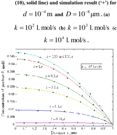
Figs. 2 to 4 represent the concentrations of the reactant

 

x

t

R

,

, product

P

 

x

,

t

, and charge carrier

n

 

x

,

t

against the distance x for various values of the rate constant. From Fig. 2, it is inferred that, when

k

less than 0.1, the concentration of reactant is uniform

i

.

e

.

R

 

x

,

t



1

for all time. Also the concentration of reactant decreases when both time t and rate constant

k

increases. The concentration of reactant has the minimum value at the electrode/polymer boundary

x



0

.

From the Fig.3, it is inferred that the concentration of product

P

 

x

,

t

increases when time

t

increases and reaches the steady-state value when

t



5 s

.

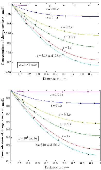
The concentration of charge carrier

n

 

x

,

t

is constant for all small values of

t



t



0 .

01 s



(see Fig. 4). For steady-state, the minimum value of the reactant

D

d

n

khR

R

x

R

ss

(

)

/

2

2 0 0 0





(3)

reactant. Similarly the maximum value of charge carrier is

n ss

x

n

khR

n

d

D

n

(

)



₀



₀ ₀ 2

/

2

at the polymer/solution interface (

x



d

). This is also confirmed in the Fig. 4a-c. Fig. 5 is the concentrations of reaction, product and charge carrier. From this figure, we can see that

   

x

,

t



P

x

,

t



1 R

for all time.

5.1. EFFECTS OF SECOND-ORDER

RATE CONSTANT

k

Second-order rate constant

k

is defined as the dimensional rate constant for the chemical reaction. In this analysis, the value of

k

is varied from

1

10



m

3

.

mol/s

to 10 m3. mol/s . Fig. 6a shows that when the process is reaction rate controlled, constant current can be predicted for higher time. However, the current increases rapidly when the value of rate constant increases.

5.2. EFFECTS OF THICKNESS OF A

POLYMER LAYER

d

Fig. 6b illustrates the effects of thickness of a polymer layer

d

on dimensional current as a function of time. It shows that current decreases slowly with increasing thickness of a polymer layer until it reaches asymptotically constant.

5.3. EFFECTS OF DIFFUSION

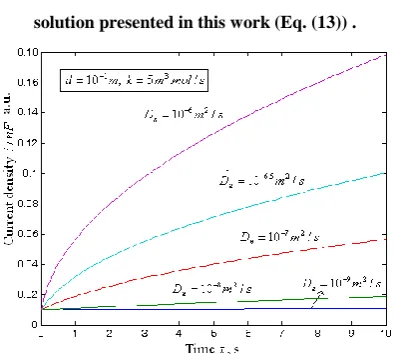
CO-EFFICIENT

D

n

Three values for the diffusion co-efficient of charge carriers

D

n_of

10

9_,

10

10_and

10

11

m

2

/s

_{have been}

considered. Fig. 6c shows the effects of diffusion co-efficient on the current as a function of time

t

/

s

for

.mol/s

m

5

3



k

_{. From Fig. 6c, it is confirmed that the}

current increases when the diffusion co-efficient

D

n

[image:3.595.320.513.78.387.2]

increases. When

D

n



8

_{the current attains the zero value.}

Fig. 2. Influence of time t on the concentration profile of

reactant

R

(

x

,

t

)

obtained from our analytical result (Eq. (10), solid line) and simulation result (‘+’) for

m

10

4



d

and

D



10

8

μm

. (a)

mol/s

l.

10

2



k

(b)

k



10

3

l.

mol/s

(c)

mol/s

l.

10

4



[image:3.595.316.516.428.658.2]

(4)

[image:4.595.330.526.73.401.2]

Fig.3. Influence of time t on the concentration profile of

product

P

(

x

,

t

)

obtained from our analytical result (Eq. (11), solid line) and simulation result (‘+’) for

m

10

4



d

and

D



10

8

μm

. (a)

mol/s

l.

10

2



k

(b)

k



10

3

l.

mol/s

(c)

mol/s

l.

10

4



k

.

Fig. 4. Influence of time t on the concentration profile of

charge carrier

n

(

x

,

t

)

obtained from our analytical result (Eq. (12), solid line) and simulation result (‘+’) for

m

10

4



d

and

D



10

8

μm

.(a)

k



10

2

l.

mol/s

(b)

k



10

3

l.

mol/s

(c)

k



10

4

l.

mol/s

.

[image:4.595.70.263.75.405.2]

Fig. 5. Concentration profiles for the reactant

R

 

x

,

t

, product

P

 

x

,

t

, and charge carrier

n

 

x

,

t

against the

distance x for

d



10

4

m

,

D



10

8

μm

and

[image:4.595.316.519.458.669.2]

(5)

[image:5.595.68.264.85.238.2]

Fig. 6a. Influence of second-order reaction rate constant k

on the current density

i

/

nF

obtained from our analytical result presented in this work (Eq. (13) ) for the

[image:5.595.69.269.297.467.2]

values of

d



10

4

m

and

D

_n



10

8

μm

.

Fig. 6b. Influence of thickness of a polymer layer

d

on

the current density

i

/

nF

obtained from our analytical solution presented in this work (Eq. (13)) .

Fig. 6c. Influence of diffusion co-efficient

D

_n on the current density

i

/

nF

obtained from our analytical

solution presented in this work (Eq. (13))

6. CONCLUSIONS

In this work, we have presented approximate analytical expressions of concentration profiles for all values of rate constant

k

. Time-dependent non-linear reaction diffusion equations have been solved analytically. The closed analytical expressions of concentrations and current are obtained using Homotopy analysis method. An agreement with the numerical result is noted. These analytical results will be useful to optimization of reaction parameters and to find the optimum efficiency of reactant to product conversion.

7. ACKNOWLEDGEMENTS

This work was supported by the Department of Science and Technology (DST), New Delhi, Government of India. The authors are also thankful Dr. R. Murali, The Principal and Mr. M.S Meenakshisundaram, The Secretary, The Madura College, Madurai for their encouragement.

8. REFERENCES

[1] Shriakawa H., (2001) The discovery of polyacetylene film:The dawning of an era of conducting polymers, Synth. Metals. 125,3.

[2] MacDiarmid A. G., (2001) Synthetic metals: a novel role for organic polymers, Synth. Metals. 125, 11.

[3] Heeger A. J., (2001) Semiconducting and metallic polymers: the fourth generation of polymeric materials, Synth. Metals. 125, 23.

[4] Wring S. A. and Hart J. P., (1992) Chemically modified, carbon paste electrodes and their application as electrochemical sensors for the analysis of biologically important compounds. A review, Analyst. 117, 1215. [5] (a) Karyakin A. A., Bobrova O. A., and Karyakina E. E.,

(1995) Electroreduction of NAD+ to enzymatically active NADH at poly (neutral red) modified Electrodes, J.Electroanal. Chem. 399, 179; (b) Karyakin A. A., Gitelmacher O. V. and Karyakina, (1995) Prussian blue-based first generation biosensor A sensitive amperometric electrode for glucose, Anal. Chem. 67, 2419.

[6] Bartlett P. N., Birkin P. R. and Wallace E. K. N., (1997) Oxidation of β-nicotinamide adenine dinucleotide (NADH) at poly(aniline)-coated electrodes, J. Chem. Soc. Faraday. Trans. 93, 1951.

[7] Lyons M. E. G., (1994) Electrocatalyis using electroactive polymers, electroactive composites and microheterogeneous systems, Analyst. 119, 805.

[8] Malinauskas A., (1999) Electrocatalysis at conducting polymers, Synth. Metals. 107, 75.

[9] Ramanaviˇcius A., Ramanaviˇcien˙e A., Malinauskas A., (2006) Electrochemical sensors based on conducting polymer-polypyrrole, Electrochim. Acta. 51, 6025. [10] Naujikas R., Malinauskas A., Ivanauskas F., (2007)

Modeling of electrocatalytic processes at conducting polymer modified electrodes, J. Math. Chem. 42, 1069.

[11] Liao S.J., Tan Y., (2007) A general approach to obtain series solutions of nonlinear differential equations, Studies in Applied Mathematics. 119, 297-354. [12] Liao S.J., (1992) The proposed Homotopy analysis

[image:5.595.69.267.501.678.2]

(6)

[13] Liao S.J., (2010) An optimal Homotopy-analysis approach for strongly nonlinear differential equations, Comm. Non-linear. Sci. Numer. Simulat. 15, 2003-2016. [14] Awawdeh F., Jaradat H. M., Alsayyed O., (2009) Solving

system of DAEs by Homotopy analysis method, Chaos, Solitons and Fractals. 42, 1422-1427.

[15] Jafari H., Chun C., Seifi S., Saeidy M., (2009) Analytical solution for nonlinear gas dynamic equation by Homotopy analysis method, Appl. Math. 4, 149-154. [16] Sohouli A. R., Famouri M., Kimiaeifar A., Domairry G.,

(2010) Application of Homotopy analysis method for natural convection of Darcian fluid about a vertical full cone embedded in pours media prescribed surface heat flux, Comm. Nonlinear. Sci. Numer. Simulat. 15, 1691-1699.

[17] Domairry G., Fazeli M., (2009) Homotopy analysis method to determine the efficiency of convective straight fins with temperature-dependent thermal conductivity, Comm. Nonlinear. Sci. Numer. Simulat. 14, 489- 499. [18] Liao S. J., On the Homotopy analysis method for

non-linear problems, Appl. Math. Comput. 147 (2004) 499-513.

[19] Domairry G., Bararnia H., (2008) An approximation of the analytic solution of some nonlinear heat transfer equations: A Survey by using Homotopy analysis method, Adv. Studies Theor. Phys. 2, 507-518. [20] Liao S. J., (2003) Beyond Perturbation: Introduction to

the Homotopy analysis method. 1st Edn. Chapman and Hall, CRC

Press, Boca Raton, p: 336. APPENDIX A

Basic idea of Liao’s [20] Homotopy analysis method (HAM) Consider the following differential equation [20]:

0 )]

(

[

u

t



N

(A1) where, Ν is a nonlinear operator, t denotes an independent variable, u(t) is an unknown function. For simplicity, we ignore all boundary or initial conditions, which can be treated in the similar way. By means of generalizing the conventional homotopy method, Liao constructed the so-called zero-order deformation equation as:

)]

;

,

(

[

)

(

)]

(

)

;

,

(

[

)

1 (



p

L



x

t

p



u

₀

t



phH

t

N



x

t

p

(A2) where p



[0,1] is the embedding parameter, h ≠ 0 is a nonzero auxiliary parameter, H(t) ≠ 0 is an auxiliary function, L is an auxiliary linear operator,

R

0

(

x

,

t

)

is an initial guess of

R

(

x

,

t

)

and



(

x

,

t

:

p

)

is an unknown function. It is important, that one has great freedom to choose auxiliary unknowns in HAM. Obviously, when

p



0

and

p



1

, it holds:

)

,

(

)

0 ;

,

(

x

t



R

₀

x

t



and



(

x

,

t

;

1 )



R

(

x

,

t

)

(A3)

respectively. Thus, as p increases from 0 to 1, the solution

)

;

,

(

x

t

p



_{varies from the initial guess}

R

₀

(

x

,

t

)

to the

solution

R

(

x

,

t

)

. Expanding



(

x

,

t

;

p

)

in Taylor series with respect to p, we

have:











1

0

(

,

)

(

,

)

;

,

(

m

m m

x

t

p

R

t

x

R

p

t

x



(A4) where

0

|

)

;

,

(

!

1 )

,

(

_





m p

m m

p

t

x

m

t

x

R



(A5) If the auxiliary linear operator, the initial guess, the auxiliary parameter h, and the auxiliary function are so properly chosen, the series (A4) converges at p =1 then we have:











1

0

(

,

)

(

,

)

,

(

m

x

t

R

t

x

R

t

x

R

. (A6) Define the vector

}

,...,

,

{

₀ ₁ _n

n

R





(A7) Differentiating Eq. (A.2) for m times with respect to the embedding parameter p, and then setting p = 0 and finally dividing them by m!, we will have the so-called mth-order deformation equation as:

)

(

)

(

]

[

₁ 1











_m _m _m m

m

R

hH

t

R

L



(A8) where

0 1

1

|

)]

;

,

(

[

)!

1 (

1 )

(

_ _

 











_m m m _m _p

p

t

x

N

m

R



(A9)

and













.

1 1,

,

1 ,

0 m

m



(A10) Applying

L

1 on both side of equation (A8), we get

)]

(

)

(

[

)

,

(

)

,

(

1

1 1

  









m m m m

m

x

t

R

x

t

hL

H

t

R



(A11) In this way, it is easily to obtain

u

m for

m



1 ,

at

M

th order, we have





M m

m

x

t

R

t

x

R

0

)

,

(

)

,

(

(A12) When

M





, we get an accurate approximation of the original equation (A1). For the convergence of the above method we refer the reader to Liao [20]. If equation (A1) admits unique solution, then this method will produce the unique solution. If equation (A1) does not possess unique solution, the HAM will give a solution among many other (possible) solutions.

APPENDIX B

Approximate solutions of the Eqs. (2) and (4) using Homotopy analysis method

(7)









_

























)

;

,

(

)

;

,

(

)

;

,

(

)

;

,

(

)

;

,

(

)

;

,

(

)

1 (

2 2

p

t

x

p

t

x

k

t

p

t

x

p

t

x

D

ph

t

p

t

x

p

t

x

D

p





(B1)









_

























)

;

,

(

)

;

,

(

)

;

,

(

)

;

,

(

)

;

,

(

)

;

,

(

)

1 (

2 2

p

t

x

p

t

x

k

t

p

t

x

p

t

x

D

ph

t

p

t

x

p

t

x

D

p

n n







(B2) where p



[0,1] is an embedding parameter and h ≠ 0 is the so-called convergence control parameter . Using Eqs. (5) to (7) we have

 

0 ,

x



R

0

,



 

0 ,

x



n

0



. (B3)

 

_{ }

.

0 ,

,

0

0 ,

0

n

t

x

t







_

(B4)

 

,

₀

,

 

,



0 .





x

d

t

R

d

t





(B5) When

p



0

0 )

0 ;

,

(

)

0 ;

,

(

2











t

x

t

x

D



(B6)

0 )

0 ;

,

(

)

0 ;

,

(

2











t

x

t

x

D

_n



(B7) By using Laplace transform method and using the boundary conditions (B3) to (B5) the solution of the above equation becomes 0

)

0 ;

,

(

x

t



R



(B8) 0

)

0 ;

,

(

x

t



n



(B9) When

p



1

the Eqs. (B3) and (B4) is equivalent to Eqs. (B1) and (B2), thus it holds

)

,

(

)

1 ;

,

(

x

t



R

x

t



(B10)

)

,

(

)

1 ;

,

(

x

t



n

x

t



(B11) Expanding



(

x

,

t

;

p

)

and



(

x

,

t

;

p

)

in Taylor series with respect to the embedding parameter p, we have,

m m

m

x

t

p

R

t

x

R

p

t

x

,

;

)

(

,

)

(

,

)

(

1 0



 







(B12) m m

m

x

t

p

n

t

x

n

p

t

x

,

;

)

(

,

)

(

,

)

(

1 0



 







(B13) where

)

0 ;

;

(

)

,

(

and

)

0 ;

;

(

)

,

(

₀

0

x

t

x

t

n

x

t

x

t

R









and

R

m

(

x

,

t

)

and

n

m

(

x

,

t

)



m



1,2,...



_{will be}

determined later. Note that the above series contains the convergence control parameter h. Assuming that h is chosen

so properly that the above series is convergent at

p



1

. We have the solution series as











1

0

(

,

)

(

,

)

,

(

m

x

t

R

t

x

R

t

x

R

(B14)



 





1

0

(

,

)

(

,

)

,

(

m

x

t

n

t

x

n

t

x

n

(B15)

where 0

)

;

(

!

1 )

,

(







p m m m

p

t

x

R

m

t

x

R

and 0

)

;

(

!

1 )

,

(







p m m m

p

t

x

n

m

t

x

n

(B16) Substituting Eq. (B14) and Eq. (B15) into the zeroth-order deformation Eqs. (B1) and (B2) and equating the co-efficient of the like powers of p we have,

1

p

: 0 0 0 2 2 0 1 2 2 1

)

1 (







hk

t

x

D

h

t

x

D

_





























(B17) 1

p

: 0 0 0 2 2 0 1 2 2 1

)

1 (





hk

t

x

D

h

t

x

D

_





























(B18) subject to the boundary conditions

 

,

0

0 ,

₁

 

,

0

1

x





x





. (B19)

 

_{ }

.

0 ,

0

1





t

x

t

_



(B20)

 

,

0 ,

1

 

,

0 .

1







x

t

d

t

d





(B21) and so on. Taking Laplace transform to the equations (B.17) and (B.18) and using the boundary conditions (B.19)- (B.21) we get

 

₂0 0

2 0 0 1

cosh

,

s

n

khR

d

D

s

x

D

s

n

khR

s

x

































(B22)

 





₂0 0

(8)

function

R

(

x

,

t

)

and

n

(

x

,

t

)

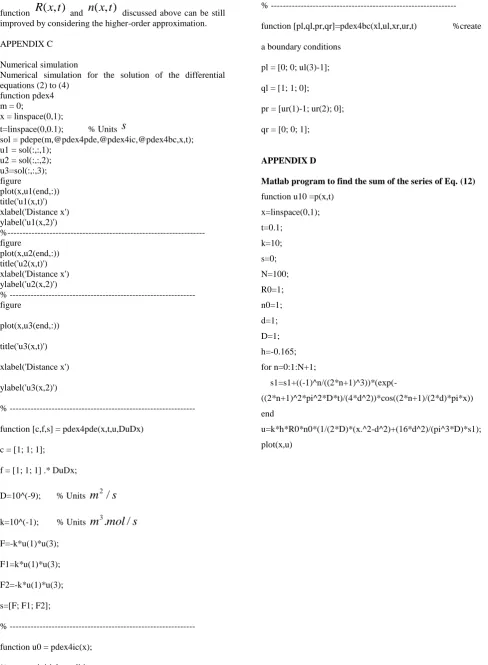
discussed above can be still improved by considering the higher-order approximation. APPENDIX C

Numerical simulation

Numerical simulation for the solution of the differential equations (2) to (4)

function pdex4 m = 0;

x = linspace(0,1);

t=linspace(0,0.1); % Units

s

sol = pdepe(m,@pdex4pde,@pdex4ic,@pdex4bc,x,t); u1 = sol(:,:,1);

[image:8.595.54.543.72.738.2]

u2 = sol(:,:,2); u3=sol(:,:,3); figure

plot(x,u1(end,:)) title('u1(x,t)') xlabel('Distance x') ylabel('u1(x,2)')

%--- figure

% --- figure

% --- function [c,f,s] = pdex4pde(x,t,u,DuDx)

c = [1; 1; 1]; f = [1; 1; 1] .* DuDx;

D=10^(-9); % Units

m

2

/

s

k=10^(-1); % Units

m

3

.

mol

/

s

F=-k*u(1)*u(3);

F1=k*u(1)*u(3); F2=-k*u(1)*u(3); s=[F; F1; F2];

% --- function u0 = pdex4ic(x); %create a initial conditions

% --- function [pl,ql,pr,qr]=pdex4bc(xl,ul,xr,ur,t) %create a boundary conditions

pl = [0; 0; ul(3)-1]; ql = [1; 1; 0];

pr = [ur(1)-1; ur(2); 0]; qr = [0; 0; 1];

APPENDIX D

Matlab program to find the sum of the series of Eq. (12) function u10 =p(x,t)

x=linspace(0,1); t=0.1;

k=10; s=0; N=100; R0=1; n0=1; d=1; D=1; h=-0.165; for n=0:1:N+1;

s1=s1+((-1)^n/((2*n+1)^3))*(exp(-((2*n+1)^2*pi^2*D*t)/(4*d^2))*cos((2*n+1)/(2*d)*pi*x)) end

(9)

NOMENCLATURE

Symbols Meaning

R

Concentration of reactant (mol m-3)

P

Concentration of product (mol m-3)

n

Concentration of charge carrier (mol m-3)

x

Thickness of a modifying layer (



m )

t

time (s)

d

Thickness of a modifying layer (



m)

D

Diffusion coefficient for reactant and product (m2s-1 )

n

D

Diffusion coefficient for charge carrier within polymer film (m2s-1 )

k

Second-order reaction rate constant (m3_{.mol s}-1₎

0

R

Concentration of reactant in the bulk solution ( mol m-3)

0

n

Concentration of charge carrier within polymer film ( mol m-3₎ I Current density (a.u.)

Table 1: Possible numerical values for parameters used in this work and Ivanauskas et al. [10] work.