Study of various motion estimation algorithms for video compression/coding standards & implementation of an optimal algorithm in LabVIEW

(1)

International Journal of Emerging Technology and Advanced Engineering

Website: www.ijetae.com (ISSN 2250-2459,ISO 9001:2008 Certified Journal, Volume 3, Issue 4, April 2013)

372

Study of various motion estimation algorithms for video

compression/coding standards & implementation of an optimal

algorithm in LabVIEW

1

Sriram B, 2Eswar Reddy M, 3Subha Varier G

1

Student, SENSE, VIT University, Vellore, Tamil Nadu, India 2

Assistant Professor, SENSE, VIT University, Vellore, Tamil Nadu, India 3

Head, Image Processing Section, Avionics Entity, VSSC, ISRO, India

Abstract— Motion estimation part is the heart of a video compression/coding standard. The compressibility factor, quality of reconstruction of frames; everything depends on the efficiency of the motion estimation algorithm that is used in the standard. In this paper seven motion estimation algorithms are discussed in detail namely Exhaustive search algorithm, Three step search algorithm, Advanced three step search algorithm, Simple and efficient three step search algorithm, Four step search algorithm, Diamond search algorithm & Adaptive rood pattern search algorithm and a comparative analysis is done using MATLAB tool. With the help of the comparative analysis, an optimal algorithm is selected based on different applications. The selected algorithm is then implemented in LabVIEW so that hardware implementation can be done as an extension work to this paper. The algorithms mentioned in this paper can be implemented in any video compression/coding standard ranging from the standard H.261 developed during 1990 to currently using high definition standard H.264.

Keywords— Video compression/coding, Motion estimation, Block matching algorithms, Mean Absolute Difference, PSNR, SSIM

I. INTRODUCTION

Currently video coding standards draw a large attention due to high storage requirements and due to the growth of internet streaming & transmission requirements. So lots of standards are developed by Video Coding Experts Group (VCEG) and Motion Picture Experts Group (MPEG) beating one over the other. At 2005, they jointly came with a high definition standard called H.264 which has gained high popularity due to its high transmission speed with low data rates and its capacity to reconstruct back the frames with maximum clarity[1],[2],[3].

[image:1.612.314.537.376.551.2]

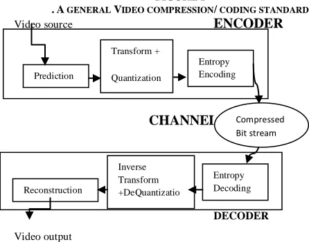
A video encoder carries out prediction, transform and encoding processes to produce a compressed bit stream and the decoder carries out the complementary processes by entropy decoding, inverse transforming and reconstructing the bit stream to produce a decoded video sequence. A general Video compression/ coding standard is shown in figure I.

FIGURE I

.A GENERAL VIDEO COMPRESSION/ CODING STANDARD

Video source ENCODER

CHANNEL

DECODER

Video output

Input to the encoding side is a sequence of consecutive frames satisfying the persistence of vision property. Frame one by one is not taken and compressed as it is. Instead, some prediction method is used that predicts frame one by one, and is subtracted with the original frame and the subtracted frame (Residual frame) is transformed, quantized and encoded to get the compressed bit stream that is either stored or transmitted depending upon the application. The same method of prediction can be done at the decoding side also to reconstruct the consecutive frames. The flow diagram for prediction block is shown in figure II.

Prediction

Transform +

Quantization

Entropy Encoding

Reconstruction

Inverse Transform +DeQuantizatio n

Entropy Decoding

(2)

International Journal of Emerging Technology and Advanced Engineering

373

FIGURE II.

FLOW DIAGRAM FOR PREDICTION BLOCK

Current Frame

Current MB Residual MB

+

-

Predicted MB

Reference Frames

Frames are processed in the form of macroblocks. The same macroblocks are predicted using prediction methods and then the original macroblock is subtracted with the predicted one to get the residual macroblock. Two types of predictions are Intra prediction and Inter prediction. Prediction done without using reference frames are called intra prediction and the prediction done using reference frames are called inter prediction. Let us discuss the prediction block in detail in frame level. Usually when the first frame comes for encoding, there will not be any reference frame. Intra prediction is done there so that some sort of frame is predicted and is subtracted with the original frame. Since prediction is done without the reference frame (intra prediction), the predicted frame may not be that much similar to the original current frame. So the residual frame will be having more information. So much compression is not there. After transforming, quantizing and encoding, the frame is reconstructed at the encoder side itself and is stored in a buffer. This frame stored in the buffer will act as the reference frame when the second frame comes for encoding. With the help of this reference frame, second frame is predicted. Since we are having a reference frame, the prediction now (inter prediction) will be more effective and the predicted frame will look more similar to the original second frame and hence the residual frame now will be having lesser information and thus more compression. Thus inter prediction proves to be more effective than intra prediction.

Thus for compression, prediction block plays an important role in such a way that more good the prediction is, more similar the original and the predicted frames will be, lesser information the residual frame will be having and thus more compression.

With this basic introduction to video compression/ coding methods, the next section explains how and why motion estimation is done. Section 3 explains the seven different motion estimation algorithms. Section 4 deals with the evaluation parameters that are used for the comparative analysis of the different algorithms. In section 5 the simulated results in MATLAB tool is discussed. Section 6 deals with the corresponding LabVIEW simulation. Section 7 explains how hardware implementation can be done as an extention work to this paper and thereby concluding this paper.

II. MOTION ESTIMATION

Assume a block in the Nth frame is moved towards its left hand side in the (N+1)th frame, it is not wise to transmit both to the receiver side as there is spatial redundancy in the two frames. For getting high compression rate, we can utilize the redundancy by sending one block‘s information and sending another information which should indicate the receiver that the same block has moved to some distance in the next frame. That extra information is the motion vector. So finding out motion vector for each and every macroblock is necessary. The process of finding motion vectors for each and every block in the current frame by finding the best match in the reference frame is called motion estimation. An example is shown in figure III where two adjacent frames are represented and a shift for a particular block is mentioned with its motion vector.

FIGURE III.

ADJACENT FRAMES INDICATING THE MOTION VECTOR Motion

Estimation Algorithm

(3)

International Journal of Emerging Technology and Advanced Engineering

374

For finding the best match, different Block Matching Algorithms (BMA) are used. The matching criterion used is Mean Absolute Difference which can be defined as shown below.

MAD =

Where C indicates the current macroblock in the current frame and R indicates the macroblock in the reference frame.

The motion estimation algorithm should produce a predicted image which should be as much similar as possible compared to the current image. Different motion estimation algorithms[4] are explained in the next section and are compared considering certain parameters.

III. MOTION ESTIMATION ALGORITHMS

A. Exhaustive Search Algorithm FIGURE IV.

THE PROCESS OF GETTING A BEST MATCH INSIDE A SEARCH AREA IN REFERENCE FRAME.

A search area of suitable size is generated in the reference frame for each and every macroblock in current frame. For a particular macroblock, searching is done and MAD values are found and the motion vector corresponding to the minimum MAD value is selected. Repeat this method for all the macroblocks in the current frame. Figure IV shows the process of getting a best match inside a search area in reference frame.

The advantage of this method is that the matching will be perfect because searching is done inside a search area which guarantees that. But it is computationally expensive. The size of search area is user defined. An example is shown in fig V.

More the search area is, more perfect the matching will be and computationally more expensive it will be. For the given example total number of search points for a macroblock is 225.

FIGURE V.

A MACRO BLOCK OF SIDE 16 PIXELS AND A SEARCH PARAMETER P OF SIZE 7 PIXELS

B. Three Step Search Algorithm FIGURE VI.

THREE STEP SEARCH PROCEDURE

(4)

International Journal of Emerging Technology and Advanced Engineering

375

The minimum MAD value among the 9 locations is found out. That location becomes the centre point for the next step and for that step, 8 surrounding locations with step size of S=S/2 is taken and again minimum MAD values are found out. Again the process continues for one more step so that S becomes 1. The location corresponding to the minimum MAD value in the final step is taken as the motion vector. In the above example, motion vector is (5,-3). The algorithm is applied for each and every macroblock of the current frame taken. Here best match is not guaranteed as in exhaustive algorithm, but the number of computations reduces to 25.

C. Advanced Three Step Search Algorithm FIGURE VII.

ADVANCED THREE STEP SEARCH PATTERN PROCEDURE

Different advancements in three step search procedures are explained in [5] and [6]. In this algorithm, along with the centre location, 16 more locations are considered in the first step i.e. 8 locations S = 4 away from the origin and 8 other locations S=1 away from the origin as shown in fig VII. If the minimum is at any of the S=1 locations, go to step 3, otherwise proceed. Step 2 is keeping the minimum point as centre, continue the three step search procedure and Goto step 1.

FIGURE VIII.

SEARCH PATTERNS FOR ADVANCED THREE STEP SEARCH ALGORITHM

(a) (b)

Step 3 is go for the neighboring points either 3 or 5 points depending on the position of the minimum at S=1 points as shown in fig 8. If the minimum MAD value point is at any one of the vertices of S=1 points, consider 5 neighboring points as in fig VIII(a) and again find the minimum MAD value and the corresponding position gives the motion vector. Otherwise take the neighboring 3 points as in fig VIII(b) and find the minimum MAD value and the corresponding position gives the motion vector.

D. Simple and Efficient Three Step Search Algorithm In this algorithm[7] first consider the 3 points A,B & C as shown in fig IX(a).

FIGURE IX.

SEARCH POINTS IN EACH QUADRANTS

Point A refers to the centre location and B & C are S=4 away from A towards right hand side and bottom. In the first step along with the 3 search points A, B & C; few more points are considered. For getting those additional points, the following conditions are checked.

If MAD(A) ≥ MAD(B) and MAD(A) ≥ MAD(C), select (b) in fig IX;

If MAD(A) ≥ MAD(B) and MAD(A) ≤ MAD(C), select (c) in fig IX;

If MAD(A) < MAD(B) and MAD(A) < MAD(C), select (d) in fig IX;

If MAD(A) < MAD(B) and MAD(A) ≥ MAD(C), select (e) in fig IX;

(5)

International Journal of Emerging Technology and Advanced Engineering

376

The location that corresponds to the minimum MAD value in the final step is taken and the coordinate shift from its original position is taken as the motion vector. The algorithm is applied for each and every macroblock of the current frame taken

FIGURE X.

SIMPLE AND EFFICIENT THREE STEP SEARCH PROCEDURE

.

An example for above algorithm is shown in fig X.The motion vector is (3,7) in the example.

E. Four Step Search Algorithm FIGURE XI.

SEARCH PATTERNS FOR FOUR STEP SEARCH

In Step 1of four step search algorithm[8], initial search location is at the centre with step size(S) = 2.

It searches the 9 locations shown in fig XI (a) and minimum MAD value is found. If minimum MAD value is at the centre goto step 4, otherwise proceed. In step 2, make the minimum MAD value point in the first step as the centre for next step and take some additional points which may be 3 or 5 depending upon the position of the selected centre point as shown in fig XI (b) & fig XI (c). i.e if the centre is at the vertex, take 5 extra points and find the minimum MAD values for that or take 3 points. If the minimum MAD value is at the centre, jump to step 4, otherwise continue. Step 3 is same as step 2.

In step 4, reduce the step size to half and again take the 8 neighboring locations (fig XI(d)) and find the minimum MAD value. Coordination vector from the centre to the minimum MAD value location gives the motion vector.

FIGURE XII.

FOUR STEP SEARCH PROCEDURE

An example for the above algorithm is represented in fig XII. The motion vector is (3,-7) in the example.

F. Diamond Search Algorithm

(6)

International Journal of Emerging Technology and Advanced Engineering

377

FIGURE XIII. DIAMOND SEARCH PROCEDURE

LDSP is applied for the initial steps. In the first step 9 locations are searched and then according to the minimum MAD value, further steps are continued. Additional locations will be either 3 or 5 depending upon the position of the minimum MAD value as shown in figure XIII. The procedure continues until we get the minimum MAD value at the centre position. Then as a last step, SDSP is applied to get the accurate least weight position.

Since the search pattern is neither big nor small and since there is no limit for the number of steps, matching will be accurate. Matching will be almost equal to exhaustive search while the number of computations will be significantly less.

G. Advanced Rood Pattern Search Pattern Algorithm

This algorithm[10] considers the fact that the motion in most of the portions in a frame will be usually homogeneous. So an adaptive searching algorithm will help a lot for the motion estimation. In this algorithm, for predicting a motion vector of a particular block, motion vector of the immediate left hand side block is taken. Consider the following example.

FIGURE XIV.

ADAPTIVE ROOD PATTERN SEARCH PROCEDURE

Assume the motion vector of a block is (3, -2). When we take the very next block, 6 locations will be considered of which the first location will be the centre point itself and the second point will be the point taken from the previous motion vector. i.e. (3,-2). Thus the searching is directly put in a point where there is the highest possibility of getting the exact match. Further, the remaining 4 points are obtained by taking a step size, S = Max (|x|,|y|). According to the example it is Max (|3|,|-2|) = 3. Thus for the first step the 6 points are as shown in the figure. If the minimum is at the centre point itself there is no further searching. Otherwise it goes to the second step where SDSP searching is done. It continues until the least weight point is obtained at the centre of the SDSP search pattern.

If the predicting vector is far away from the centre, the searching is directly put in a point where there is the highest possibility of getting the exact match, so that the number of computations can be saved to a great extend compared to other methods without trading off the best matching guarantee.

IV. EVALUATION PARAMETERS

The evaluation criterion parameters should be taken for the comparison of the algorithms in such a way that the parameters should indicate the similarity of the predicted frame with the current frame. Some of the parameters that talk about the similarity between two frames are Peak Signal to Noise Ratio (PSNR) and Structural Similarity index (SSIM). The third parameter talks about the average number of search points for a macroblock in a particular algorithm.

Predicted Vector

(7)

International Journal of Emerging Technology and Advanced Engineering

378

What we need is maximum values for PSNR and SSIM so that the predicted frame is maximally similar to the original current frame and minimum value for the average number of search points so that the algorithm can be done in real time.

A. Peak Signal to Noise Ratio (PSNR):

Peak Signal to Noise Ratio is measured on a logarithmic scale and depends on the mean squared error (MSE) between an original and an impaired image or video frame, relative to (2n −1)2 (the square of the highest-possible signal value in the image, where n is the number of bits per image sample). PSNR in dB is given by

PSNR=10 log10 (I2/MSE)

Where I is the maximum intensity level MSE – Mean Square Error

MSE =

A - Original Image

B - Reconstructed Image

M & N - size of image

B. Structural Similarity Metric Index (SSIM):

The SSIM index is the objective image quality measure and can be defined as

SSIM (A, B) =

Where A=Original Image

B=Reconstructed Image

μA & μB – mean intensities of data A & B

σA & σ B – standard deviations of data A & B

C. Average number of search points for one macroblock for the algorithm.

V. SIMULATED RESULTS

For evaluation purpose, three types of video sequences are taken; one which has generally lower motion of objects in frames (mrchest); second one with medium motion of objects (caltrain) and the third one which has random motion of objects in the frames.

The PSNR, SSIM and the number of search points for all the algorithms are taken and compared for all the 3 types of sequences and is tabulated below. The simulation is done using the Digital Signal Processing tool, ‗MATLAB‘. Table I, table II and table III shows the simulated values for caltrain, football and mrchest sequences respectively.

TABLE I:

SIMULATED VALUES FOR CALTRAIN SEQUENCE

Algorithm

PSNR (dB)

SSIM

No. of search points Theore

tical

Simula ted Exhaustive

search 32.24 0.9243 210 210.3 Three step

search 30.32 0.8935 25 23.8

Advanced 3

step search 32.18 0.9236 17-33 20.18

Simple & Efficient 3 step search

29.65 0.8732 10-16 16.33

4 step search 30.67 0.9005 17-27 18.81 Diamond

search 32.12 0.9218 13-28 15.83 Adv Rood

Pattern Search

32.05 0.9227 ~9 8.24

TABLE II:

SIMULATED VALUES FOR FOOTBALL SEQUENCE

Algorithm

PSNR

(dB)

SSIM

No. of search points

Theoret ical

Simulat ed

Exhaustive

search 23.80 0.7424 210 202

Three step

search 23.47 0.6688 25 23.12

Advanced 3

step search 23.53 0.7423

17-33

(8)

International Journal of Emerging Technology and Advanced Engineering

379

22.92 0.6565 10-16 15.75

4 step search 23.51 0.7229 17-27 19.21

Diamond

search 23.41 0.7393 13-28 18.1 Adv Rood

23.45 0.7353 ~9 10.55

TABLE III:

SIMULATED VALUES FOR MRCHEST SEQUENCE

Algorithm

PSNR

(dB)

SSIM

No. of search points

Theoret ical

Simulat ed

Exhaustive

search 42.75 0.9932 210 199.5

Three step

search 42.74 0.9931 25 22.8

Advanced 3

step search 42.74 0.9931 17-33 15.53

42.71 0.9931 10-16 16.89

4 step search 42.74 0.9931 17-27 15.53 Diamond

search 42.74 0.9931 13-28 12.02 Adv Rood

42.72 0.9931 ~9 4.93

In the above tabulations, parametric values between two adjacent frames are simulated in MATLAB. Now adjacent frames one by one is taken from the ‗caltrain‘ sequence.

When the first frame comes for encoding it is stored in a buffer so that it can be used as the reference frame when the second frame comes for encoding. Using the reference frame, through the motion estimation algorithm, second frame is predicted which should be similar to the original second frame. Second frame is stored in buffer again so that it can be used as a reference frame for third. The process is continued for 31 frames and the PSNR, SSIM & search points calculated for all those frames are plotted in figures XV, XVI & XVII respectively.

FIGURE XV.

GRAPH SHOWING PSNR VALUES FOR DIFFERENT FRAMES

FIGURE XVI.

(9)

International Journal of Emerging Technology and Advanced Engineering

380

FIGURE XVII.

GRAPH SHOWING SEARCH POINT VALUES FOR DIFFERENT FRAMES

There are certain advantages for ARPS algorithm over other algorithms. The average number of search points is least among the algorithms used preserving the PSNR & SSIM values. Also if the predicted motion vector is (0, 0), it does not waste computational time in doing LDSP, it rather directly starts using SDSP. Furthermore, if the predicted motion vector is far away from the center, then again ARPS save on computations by directly jumping to that vicinity and using SDSP.

Due to the reasons mentioned above, Adaptive Rood Pattern Search Algorithm is selected as the optimal algorithm for any type of application.

VI. LABVIEW IMPLEMENTATION

Usually for hardware implementation Hardware Descriptive Languages like VHDL, Verilog etc are used. Here LabVIEW is used since it is having certain advantages compared to former one. Studying LabVIEW tool is very easy compared to HDL. Circuit implementation is also easier in LabVIEW and is more faster compared to HDL.

LabVIEW (Laboratory Virtual Instrumentation Engineering Workbench) is a system design platform and development environment for visual programming language developed by National Instruments[11]. LabVIEW is well suited for FPGA programming because it clearly represents parallelism and data flow. Achieving high-level design with low-level ability and powerful graphical programming for FPGA Hardware are some of the key features for using this tool.

The selected optimal algorithm is implemented in LabVIEW so that hardware implementation can be done[12]. Biomedical toolkit is used which inputs the series of consecutive frames into the tool. The LabVIEW VI circuit is developed and the PSNR, SSIM and search point plots are simulated as shown in figure XVIII, XIX & XX. The simulated LabVIEW results match the MATLAB results as shown below.

FIGURE XVIII.

GRAPH SHOWING PSNR VALUES FOR DIFFERENT FRAMES

FIGURE XIX.

(10)

International Journal of Emerging Technology and Advanced Engineering

381

FIGURE XX.

GRAPH SHOWING SEARCH POINT VALUES FOR DIFFERENT FRAMES

VII. CONCLUSION AND FUTURE SCOPE

Various motion estimation techniques for video compression is studied using a comparative analysis and Adaptive Rood Pattern Search Algorithm is selected as an optimal algorithm. The selected algorithm is then implemented in LabVIEW so that hardware implementation can be done. These are the analytical conclusions in this paper. Through an interface, hardware implementation can be done in Xilinx FPGA. Hardware implementation can also be done directly without any interface in LabVIEW‘s processor cum FPGA device called CompactRIO.

VIII. ACKNOWLEDGMENT

This work was supported by Shri. Anand.K, Project Manager of Avionics & Ground Stations at Vikram Sarabhai Space Centre, Indian Space Research Organisation, India and Shyam Krihnan from Anna University, Guindy, Chennai, India.

REFRENCES

[1] Iain E.Richardson ,“The H.264 Advanced video compression standard” (Second edition), 2010, John Wiley & Sons, Ltd. [2] Study materials and tutorials from website.

http://www.vcodex.com

[3] T.Wiegand, G.J.Sullivan, G.Bjontegaard, A.Luthra, “ Overview of the H.264/AVC video coding standards”, IEEE transactions on

circuits and systems for video technology, Vol.13, No.7, July 2003.

[4] Faizul Hadi Jamil, Ali Chekima, Rosalyn R. Porle, Othman Ahmad, Norfarariyanti Parimon, “BMA Performance of Video Coding for Motion Estimation”,IEEE 2012 Third International

Conference on Intelligent Systems Modelling and Simulation,

978-0-7695-4668-1/12 DOI 0.1109/ISMS.2012.115.

[5] Renxiang Li, Bing Zeng, and Ming L. Liou, ―A New Three-Step Search Algorithm for Block Motion Estimation‖, IEEE Trans.

Circuits And Systems For Video Technology, vol 4., no. 4, pp.

438-442, August 1994.

[6] SUN Ning-ning, FAN Chao, XIA Xu, ―An Effective Three-step Search Algorithm for Motion Estimation‖, 2009 IEEE, 978-1-4244-3929-4/09.

[7] Jianhua Lu, and Ming L. Liou, ―A Simple and Efficent Search Algorithm for Block-Matching Motion Estimation‖, IEEE

Trans.Circuits And Systems For Video Technology, vol 7, no. 2, pp.

429-433,April 1997.

[8] Lai-Man Po, and Wing-Chung Ma, ―A Novel Four-Step Search Algorithm for Fast Block Motion Estimation‖, IEEE Trans. Circuits

And Systems For Video Technology, vol 6, no. 3, pp. 313-317, June

1996.

[9] Shan Zhu, and Kai-Kuang Ma, ― A New Diamond Search Algorithm for Fast Block-Matching Motion Estimation‖, IEEE Trans. Image

Processing, vol 9, no. 2, pp. 287-290, February 2000.

[10] Yao Nie, and Kai-Kuang Ma, ―Adaptive Rood Pattern Search for Fast Block-Matching Motion Estimation‖, IEEE Trans. Image

Processing, vol 11, no. 12, pp. 1442-1448, December 2002.

[11] Study materials and tutorials from website.

http://www.ni.com.