Journal of Chemical and Pharmaceutical Research, 2014, 6(4):14-22
Research Article
CODEN(USA) : JCPRC5
ISSN : 0975-7384
Preventive maintenance model analysis on repairable components
Su Hong-Sheng*, Li Juan-Di and Kang Yong-Qiang
School of Automation and Electrical Engineering, Lanzhou Jiaotong University, Lanzhou, China
____________________________________________________________________________________________
ABSTRACT
In order to provide the scientific theoretical basis for component’s maintenance and management, state transition diagram of repairable components is established, and state transition equations are achieved based on reliability mathematical theory in this paper. And then its transient process and stability is investigated. The three kinds of mathematical models are respectively established for the passive maintenance, and the preventive maintenance, and as well as the redundant maintenance, and their average maintenance cost rates are calculated for repairable components. The related investigation results show that the maintenance cost rate of preventive maintenance is the lowest, and is the optimal maintenance strategy.
Key words: State equation; transient; stability; preventive maintenance; average maintenance cost rate
____________________________________________________________________________________________
INTRODUCTION
Preventive maintenance is an important mean to improve component reliability. Since Barlow proposed minimal repairing theory, many periodic maintenance models with time-based have been established, and many servicing models to calculate fixing cycle T have already been reported [1-3]. But Khandelwal found it difficult to select the proper maintenance cycle T. For it can cause excessive maintenance so that maintenance cost increases to prolong or shorten the repairing interval[4]. Subsequently, Nguyen, Murthy and Nakagawa proposed a sequential policy where the preventive maintenance was performed in a time interval,but the varies with the age of the components[5-6]. Hence, the component maintenance models with state-based have been widely investigated since 1980s. In [7] a replacement maintenance strategy was proposed based on Markov decision process. Further, Love developed incomplete maintenance strategy where state space was component age and number of the failures [8]. However, it is difficult for these models to judge components recession correctly. In addition, the related simulation results also show certain errors compared with the actual state of components, and maintenance strategy is not for that optimal. Therefore, in this paper, the component state is divided into three groups: working state, storage state, and maintenance state. On the basis of it, the state equations are established, and its transient process and stability are analyzed. Moreover, the paper also compares repairable component’s average maintenance cost rate among passive maintenance model, and preventive maintenance model, and redundant maintenance model. The related investigation results show that the preventive maintenance scheme is best, and redundant maintenance is worst.
1. MODEL DESCRIPTIONS
To establish the life cycle model for repairable component we need to do the following assumptions.
Hypothesis 1 Component maintenance and inspection only use a state to express.
Hypothesis 2 Whether component is in working state or storage state, it is not existed for the failure that can’t be detected out.
Δt, the transfer rate is a constant which does not depend on the time t and Δt.
Hypothesis 4 Maintenance will not change failure rate of the component.
Hypothesis 5 The used failure rate function is the bathtub curve with its first stage and the aging stage being ignored. And so the failure rate is the constant.
Hypothesis 6 Preventive maintenance is perfect, i.e., if there are faults detected out during preventive maintenance, and then it would be able to get a timely repair.
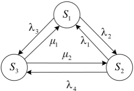
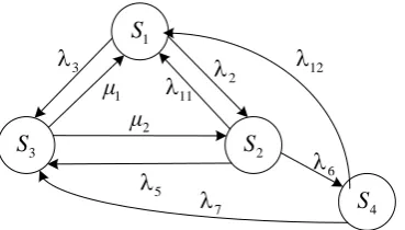
According to the assumptions mentioned above, the state transition diagram of the repairable component can be drawn out as shown in Fig. 1.
1 S
2 S 3
S
1 μ
2 μ
2
1
4
3
[image:2.595.238.374.221.313.2]
Fig. 1: State transition diagram of repairable compone nt
In Fig.1, S1 denotes that component is being in storage state, and S2 denotes that component is in working state, and S3 denotes the combined state of preventive maintenance and corrective maintenance because preventive
maintenance time is considered to be same with corrective maintenance time, here we assume that preventive maintenance can accomplish an eventual substitution before there is an upcoming failure or after a random damage happens, and λ1 is the transition probability from working state to storage state, and λ2 is the transition probability
from storage state to working state, and λ3=v1+u1, where v1 and u1 denote respectively the failure rate and the
checking rate of the stored component, and λ4=v2+u2, where v2 and u2 denote respectively the failure rate and the
checking rate of the working component, and μ1 is the stored probability after one maintenance; μ2 is the used
probability after one maintenance.
2. MATHEMATICAL MODEL ANALYSIS
According to Fig. 1, and reliability theory[9, 10], we can get
1
1 2
2 3 1 1 3
2
1 2 3
2 1 4 2
3
1 2 3
3 4 1 2
1 2 3
d ( )
( ) ( ) ( ) ( )
d ( )
( ) ( ) ( ) ( )
d ( )
( ) ( ) ( ) ( )
( ) ( ) ( ) 1, 0. x t
x t x t μ x t
λ λ λ
dt x t
x t λ x t μ x t
λ λ
dt x t
x t x t μ μ x t dt
x t x t x t t
(1)
where x1(t) denotes the probability of being in the state S1 at time t, and x2(t) denotes the probability in S2, and x3(t)
is the probability S3. The above differential equations can be written as
1
d ( ) / d
x
t
t
A x
( )
t
μ
(2)1 1 1 1 2 3 1 1 1
1
2 2 2 2 2 2 1 4 2
1 2
( )
,
,
( )
,
.
.
( )
,
( )
( ) 1,
0; 0
, (
1, 2,3, 4); 0
i; (
1, 2)
d
a
x t
μ
d
μ a
μ
=
t
b
d
x t
μ
b
μ d
μ
x t
x t
t
i
μ
i
i
A
x
μ
According to linear systems theory[11], if the matrix A1 satisfies d1d2–ab>0, the system (2) would be stable. When t
_____________________________________________________________________________
1 1 1
2 ( ) ( )
( ) x =
x
x A μ
Thus, the solution of the linear system (2) can be written as
1
( )
t
exp(
)[ (0)
( )
] +
( )
x
A t x
x
x
(3)Where x(0) is the initial value. From (3), the transient process of x(t) is mainly decided by matrix exponent function exp(A1t). In other words, it is determined by the eigenvalues of A1. The eigenvalues of the matrix A1 can be resolved
by
1 1 2
2 1 2
(
) 2
2
(
) 2
2
s
d
d
s
d
d
Where
(
d
1
d
2)
2
4
ab
s
2s
1As Δ>0, the matrix has two different negative eigenvalues. It is easy to known that the A1 has similarity matrix, i.e.,
there exists an invertible matrix P meeting P-1A1P = B which is formed by eigenvectors corresponding eigenvalues
of A1, and so exp(A1t)=Pexp(Bt)P-1[12], where Bis a diagonal matrix of its diagonal elements being s1 and s2. Then
we have
1 2 2 1
2 1 1 2
11 12
1 2 1 1
1
21 22
2 2 2 1
2 1
( )
( )
(
)
(
)
(
)
1
exp(
( )
( )
(
)
(
)
(
)
s t s t s t s t
s t s t s t s t
a
t
a
t
d
s e
d
s e
a e
e
)=
a
t
a
t
b e
e
d
s e
d
s e
s
s
A t
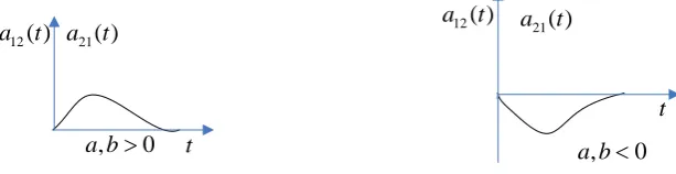
The motion track of a12(t) and a21(t) are mainly determined by the es2t-es1t. Its motion curves can be shown as Fig.2.
t
t 12( )
a t a12( )t
, 0
a b a b, 0
21( )
[image:3.595.88.529.360.398.2]a t a21( )t
Fig. 2: Motion curves of non-diagonal elements
For a11(t) and a22(t), if ab>0((d1-d2)2+4ab>0), a11(t) and a22(t) are all monotonically decreasing, its motion curves
can be shown as Fig.3. Otherwise, if ab<0( d1d2 2 ab), both of them are not monotonically decreasing, as specified in Tab.1.
t 11( )
a t a22( )t
[image:3.595.150.457.444.523.2]Table 1 Motion curves of diagonal elements(ab<0)
a11(t) a22(t)
1
d
>d
2
2
ab
2
d
>d
1
2
ab
As Δ=0(
d
1
d
2
2
ab
), the A1 has two same negative real eigenvalues, that is s=s1=s2=
(
d
1
d
2) 2
.Clearly,d1d22 ab, and then we have
s s
11 12
1 2
1 s s
21 22
2 1
( )
( )
[1 (
) 2]
exp(
) =
( )
( )
[1 (
) 2]
t t
t t
b t
b t
e
d
d t
ate
t
b
t
b
t
bte
e
d
d t
A
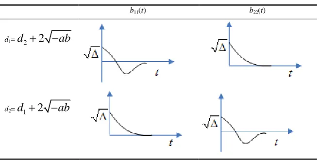
For b12(t) and b21(t), their motion curves are mainly determined by the test, and is similar as Fig.2. For b11(t) and b22(t), its motion curves are specified as the Tab. 2.
Table 2 Motion curves of diagonal elements
b11(t) b22(t)
d1=
d
2
2
ab
d2=
d
1
2
ab
As Δ<0(
d
1
d
2
2
ab
), the matrix’s eigenvalues are two conjugate imaginary roots, i.e.1 1 2
2 1 2
(
) 2
j
2
j
(
) 2 + j
2
j
s
d
d
α
β
s
d
d
α
β
Thus we have exp(A1t)= P1 exp(B1t) P1-1.
Where 1 1 1
1 2
0
cos
sin
2
,
, exp(
)
sin
cos
2
(
) 2
t
a
α
β
βt
βt
=
t
e
β α
βt
βt
a
d
d
α
[image:4.595.143.472.414.580.2]_____________________________________________________________________________
And so
1 2 11 12
1
21 22
1 2
cos ( ) sin 2 sin ( ) ( )
exp( )
( ) ( )
2 sin cos ( ) sin
t βt d d βt a βt c t c t
e t
c t c t
b βt βt d d βt
α
A
The motion track of c12(t) and c21(t) are mainly determined by the
sin
.
t
[image:5.595.72.288.340.412.2]e
βt
Its motion curves can be shown as Fig.4.t
12
( )
c
t
21
( )
c
t
,
0
a b
t
12
( )
c
t
21
( )
c
t
,
0
a b
Fig. 4: Motion curves of non-diagonal elements
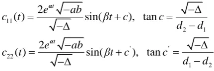
For c11(t) and c22(t), they can be simplified as
11
2 1
' '
22
1 2
2
( )
sin(
), tan
2
( )
sin(
), tan
t
t
e
ab
c
t
βt c
c
d
d
e
ab
c
t
βt c
c
d
d
α
α
Their motion tracks are similar to Fig.4, and the initial phases are different alone.
From what has been discussed above, as long as the eigenvalues of the matrix A1 possess negative real parts, then
1 lim exp( )
t At 0. In other words, the system (3) is stable.
3. STABILITY ANSLYSIS WITH TIME-VARIABLE SYSTEM
For system (2), if A1 is independent of time, and whose eigenvalues have negative real parts, the system is then
stable. If A1 relies on time, its stability needs to make study, further. If the checking rates of matrix A1 change with
time while others keep invariant, A1 can be then written as
1
( )
t
A = A + U
where 3 3 2 1 1 1 1 1
4 2 2 4 1 2 2 2
,
( )
0
,
.
( )
,
0
( )
d
a
d
v
μ a
μ
u t
t
b
d
b
μ d
v
μ
u t
A =
U
For conveniently analysis, we first make the following definitions. (1) The mark‖•‖stands for the norm of vectors or matrices.
(2) eAt can be expressed by
ij( )
t
, andeA(t-τ) can be expressed by
ij( - ),
t
i j
,
1 2
,
Theorem 1. For linear time-variable system
d ( ) / d
x
t
t
A + U
( )
t
x
( )
t
(4)having that
1 2
0 u t( ) u t( ) dt
if d ( ) / dx t tAx( )t is asymptotically stable, system (4) is asymptotically stable.
Proof. The solution of system (4) is
0
0
( ) ( )
0
( )
t t t t( ) ( )
t
t
e
A
e
A
d
x
x
U
x
Hence, we have
0
0
2 )
0 1 2
j 1
( )
( t t t ij(
)
( )
( )
( )
t i
t
e
t
τ
u τ
u τ
τ d
A
x
x
x
、
(5)
Since d ( ) / dxt tAx( )t is stable, let ( 0)
0 t t
e
A x
≤K, we have2
j 1
(
)
ij i
t
τ
L
、
t
0
τ t
. LetM=max(K, L), so we have
0
1 2
( )
t( )
( )
( )
t
t
M
M
u τ
u τ
τ d
x
x
(6)Let u(τ)=u1(τ)+u2(τ), then substituting it into (6) , we have
0
( )
( )
( )
1
t( )
( )
t
t u t
Mu t
u τ
τ dτ
x
x
Then integrating from t0 to t, we have
0
0ln 1
t( )
( ) d
t( )
t
u τ
τ
τ
M
tu τ dτ
x
(7)And so,
x
( )
t
can be written as0
0
( )
1 2
( )
( )
( )
( )
t t
M u τ dτ
t
t
t
M
M
u τ
u τ
τ dτ Me
x
x
(8)Hence, if
1 2
0
u t
( )
u t dt
( )
<∞,thenx
( )
t
is bounded, system (4) is stable. In another hand, ifd ( ) / d
x
t
t
Ax
( )
t
is asymptotically stable, thenlim
00
tt
e
A
x
, and0
lim
t( )d
t
t
M
u τ
τ
0
0
( )d
t
u τ
τ
=0×bounded function =0. Thus, we obtain 0( )
( )
0 1 0
t t
M u τ dτ
t
Me
x
.And therefore, system (4) is also asymptotically stable.
4. MAINTENANCE MODEL ANALYSIS
In Fig.1, if u1=0, u2=0, then λ3=v1, λ4=v2, and then, the system (4) shows the passive maintenance. Then equation (2)
can be written as
11
_____________________________________________________________________________
Where 11 11 1 1 11 2 1 1 1 1
22 2 2 2 2 22 1 2 2
( )
,
, ( )
,
.
.
( )
,
d
a
x t
μ
d
v
μ a
μ
t
b
d
x t
μ
b
μ d
v
μ
A =
x
μ
As t→∞, the steady state value of the system is
1 2 1 1 2
1
1 2 1 2 1 1 2 2 1 2 1 2 2 1
2 1 2 2 1
2
1 2 1 2 1 1 2 2 1 2 1 2 2 1
(
)
( )
(
)(
)
+
(
)
( )
(
)(
)
+
+ v μ
μ
x
μ
μ
v
v
v v
v μ
v μ
v μ
μ
x
μ
μ
v
v
v v
v μ
v μ
(10)
When the system being at steady-state, and in range of time T, let the time being in state S1, S2 respectively be T1, T2,
and then
1 1
( ),
2 2( )
T
Tx
T
Tx
(11)Let C be a component cost, and Cm1 is the component’s desired storage cost per unit time, and N be the component’s
expected number of failures on the scope of time T, thus we have
1 2
1 2 1 1 2 2
0 0
=
T TN
v dt
v dt
T v
T v
(12)If a component failure occurs it will be replaced using new one. So average maintenance cost rate during time T can be written as
1 1
1 1 1
( )
1( )
1 2( )
2m
m
C T
CN
f
C x
C x
v
x
v
T
(13)If u1≠0, u2≠0, λ3= u1+v1, λ4= u2+v2, Fig.1 stands for the preventive maintenance model of component. When t→∞,
the steady state value of the system is
1 4 1 4 2
1
1 2 1 2 1 3 2 4 3 4 3 2 4 1
2 3 2 2 1
2
1 2 1 2 1 3 2 4 3 4 3 2 4 1
1 3 2 4 3 4
3
1 2 1 2 1 3 2 4 3 4 3 2 4 1
(
)
( )
(
)(
)
+
(
)
( )
(
)(
)
+
+
( )
(
)(
)
+
+
μ
μ
x
μ
μ
μ
μ
μ
μ
x
μ
μ
μ
μ
x
μ
μ
μ
μ
(14)
In the preventive maintenance period, if component is in failure, then we perform minimal repairs (repaired as old). At steady state, during time T, the time being in state S1, S2, and S3 is T1’, T2’, and T3’,respectively. Therefore
' ' '
1 1
( ),
2 2( ),
3 3( )
T
Tx
T
Tx
T
Tx
(15)Let Cm2 be the component’s desired storage cost per unit time, and Cr2 is the minimal repair cost for each
time(ignoring minimal repairs’ repairing time), and Cf2 be the component’s desired preventive maintenance cost per
unit time, N’be the component’s expected number of failures during time T, thus
' '
1 2
' ' '
1 2 1 1 2 2
0 0
=
T TSo the average maintenance cost rate in T can be written as
' ' '
2 1 2 2 3
2 2 1
( )
2 1( )
1 2( )
2 2 3( )
m r f
m r f
C T
C N
C T
f
C x
C
x
v
x
v
C x
T
(17)
When there is redundant spare working component, a state S4 is increased as shown in Fig.5 [14]. At this moment, S2
represents one component in the working state and the other is spare component. S4 represents the working
component for repairing or entering the warehouse storage, while spare component works.
1 S
2 S 3
S
4 S 1
μ
2 μ
2
11
12
6
7
3
5
[image:8.595.216.401.190.295.2]
Figure 5: The state transition diagram with redundant component
The state transition equation is
33 1
d ( ) / d
x
t
t
A x
( )
t
μ
(18) where' '
11 1 2 1 1 11 2 3 1 1 11 1 2 12 1
' '
33 22 2 2 1 2 2 2 22 11 5 6 2
6 33 4 33 12 7
( )
,
,
, ( )
( ) ,
.
,
0
( )
0
d
a
a
x t
μ
d
μ a
μ a
μ
b
d
-μ
t
x t
μ
b
μ d
μ
d
x t
d
A =
x
μ
As t→∞, the steady state value of the system is
'
22 33 6 2 1 1 33 2 6 2
1 ' ' '
11 22 33 2 1 6 11 6 2 33 1 1
'
1 33 1 11 33 2
2 ' ' '
11 22 33 2 1 6 11 6 2 33 1 1
'
1 6 1 11 6 2
4 ' ' '
11 22 33 2 1 6 11 6 2 33 1 1
3 1
(
)
(
)
( )
( )
( )
( ) 1
d d
μ μ
a d
a
μ
x
d d d
a b
d
μ
d a b
b d μ
d d μ
x
d d d
a b
d
μ
d a b
b
μ
d
μ
x
d d d
a b
d
μ
d a b
x
x
( )
x
2( )
x
4( )
(19)
When being at steady state, during time T, let the time being in state S1, S2, S3, and S4 be T1”, T2”, T3”,and T4 ” ,
respectively. Then
'' '' '' ''
1 1
( ),
2 2( ),
3 3( ),
4 4( )
T
Tx
T
Tx
T
Tx
T
Tx
(20)Let C be component cost, and Cm3 be the component’s desired storage cost per unit time, and Cf3 be the component’s
desired preventive maintenance cost per unit time, and N’’be the component’s expected number of failures during time T, thus
'' '' ''
1 2 4
'' T
T
T
''
''
''_____________________________________________________________________________
If a component failure occurs, it will be replaced with the new. So average maintenance cost rate during time T can be written as
'' '' ''
3 1 3 3
3 3 1
( )
1( )
1 2( )
2 7 4( )
3 3( )
m f
m f
C T
CN
C T
f
C x
C x
v
x
v
x
C x
T
(22)5. EXAMPLE
The transition rates per month of the parameters of the production devices of an enterprise are given as follows: λ1=
1.5625, λ2= 1.875, v1= 0.0020, v2= 0.0020, μ1=1.2500, μ2=0.6250, u1= 1.2500, u2= 0.6250, λ5=0.4685, λ6= 1.2500,
λ7= 0.4685, λ11=0.7813, λ12= 0.7813[14].
Let C be the component cost. In the first model, let Cm1=0.01C. According to parameters given above, we have x1(∞)=0.4542, and x2(∞)=0.5448, and so average maintenance cost rate f1 is 0.006542C during time T.
In the second model, let Cm2=0.01C,Cr2=0.01C, Cf2=0.01C. According to parameters given above, we have x1(∞)=0.3113, and x2(∞)=0.3603,and x3(∞)=0.3284, so average maintenance cost rate f2 is 0.006398C during time T.
In the third model, let Cm3=0.01C,and Cf3=0.01C. According to parameters given above, we have x1(∞)=0.2318, and x2(∞)=0.2405, and x3(∞)=0.2663, x4(∞)=0.2614, so average maintenance cost rate f3 is 0.126421C during time T.
From the above calculation, we have f2f1f3. Clearly, the average maintenance cost rate of preventive maintenance
scheme is the lowest, and the highest for redundant maintenance. The main reason for this result lies in that the model 1 and the model 3 adopt corrective maintenance, while model 2 adopts preventive maintenance. Therefore, it is easy to draw conclusion that preventive maintenance model is the best model for some repairable components.
CONCLUSION
This paper firstly analyzes transient process and stability of state equation of repairable components. Secondly, three different maintenance models are introduced. At last the average maintenance cost rates of all models are calculated. The above study can provide the theoretical basis for system operation and maintenance, helping people make scientific, reasonable production plans and maintenance works. It is necessary for enterprise to build optimal model that can help its manager make the decision to obtain maximum profit.
Acknowledgments
This project is supported by the National Natural Foundation of China (Grant No.61263004) and Gansu Province Natural Science Foundation (Grant No.1212RJZA071).
REFERENCES
[1] Barlow R, Hunter L. Operations Research, v.8, n.1, pp. 90-100, 1960. [2] Canfield, R. IEEE Transactions on Reliability, R35(1), pp. 78-81, 1986.
[3] Grigoriev Alexander, Van de Klundert Joris, Spieksma Frits C. R. European Journal of Operational Research, v.172, n.3, pp. 783-797, 2006.
[4] Khandelwal D N, Sharma J. Ray L M. IEEE Trans Automatic Control, v.24, n.3,pp.513-513, 1979. [5] Nguyen & Murthy. IEEE Transactions on Reliability, R26(3), pp. 1181-1194, 1981.
[6] Nakagawa. IEEE Transactions on Reliability, v.137, n.3, pp. 295-298, 1988.
[7] Shey-HueiSheu, WilliamS.Griffith. IEEE Transactions on Reliability, v.50, n.3, pp. 302-309, 2001.
[8] Love C E, Zhang Z G, Zitron M A. European Journal of Operations Research, v.25, n.2, pp. 398-409, 2000. [9] Cao Jinhua, Cheng Kan. Reliability Mathematical Introduction, pp. 182-244, 2006.
[10]Su Hongsheng. Journal of Zhejiang University(Engineering Science), v.44, n.7, pp. 136-145, 2010. [11]DRIELS M. Linear control systems engineering, pp.164-242, 1996.
[12]Zheng Dazhong. Linear system theory, pp. 90-95, 2002.
[13]Qian Xuesheng, Song Jian. Engineering Cybernetics, pp. 127-133, 2011.