PAPER • OPEN ACCESS
The analysis of morphometric data on rocky
mountain wolves and artic wolves using statistical
method
To cite this article: Muhammad Ammar Shafi et al 2018 J. Phys.: Conf. Ser. 995 012015
View the article online for updates and enhancements.
Related content
NOTES ON COMET 1916, (WOLF) R. T. Crawford
-THE PERTURBATION OF WOLF 1062. R. S. Harrington
-PERIODIC COMET WOLF I W. Baade
-1
Content from this work may be used under the terms of theCreative Commons Attribution 3.0 licence. Any further distribution of this work must maintain attribution to the author(s) and the title of the work, journal citation and DOI.
Published under licence by IOP Publishing Ltd
The analysis of morphometric data on rocky mountain wolves
and artic wolves using statistical method
Muhammad Ammar Shafi1, Mohd Saifullah Rusiman1, Nor Shamsidah Amir Hamzah1, Maria Elena Nor, Noor’ani Ahmad1, Nur Azia Hazida Mohamad Azmi1, Muhammad Faez Ab Latip2, Ahmad Hilmi Azman2
1Faculty of Science, Technology and Human Development, Universiti Tun Hussein
Onn Malaysia, 86400 Parit Raja, Batu Pahat, Johor, Malaysia.
2Faculty of Science Computer and Mathematics, Universiti Teknologi Mara, Jabatan
Universiti Kota Bharu, Kelantan, Malaysia
E-mail: [email protected], [email protected]
Abstract.Morphometrics is a quantitative analysis depending on the shape and size of several specimens. Morphometric quantitative analyses are commonly used to analyse fossil record, shape and size of specimens and others. The aim of the study is to find the differences between rocky mountain wolves and arctic wolves based on gender. The sample utilised secondary data which included seven variables as independent variables and two dependent variables. Statistical modelling was used in the analysis such was the analysis of variance (ANOVA) and multivariate analysis of variance (MANOVA). The results showed there exist differentiating results between arctic wolves and rocky mountain wolves based on independent factors and gender.
1. Introduction
[image:2.595.161.435.570.723.2]Morphometrics is quantitative analysis based on size and shape specimens’ concept [1]. Morphometric analyses are basically used on organisms, fossil record, mutations on shape and others. Morphometrics can be used to find the significance level of specimens, changing in shape of size specimens and relationship between same species of specimens or different species of specimens [4]. A major function of morphometrics is to confirm hypotheses about shape and size utilising statistical technique.
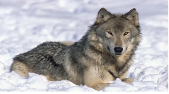
The Northern Rocky Mountains wolf also known asCanis lupusis a subspecies of the gray wolf from western United States by 1930s. This species population grew from 60 wolves in 1994 to 1704 wolves in 2015 at Montana, Idaho. The wolf population continued to grow in Oregon and Washington [2, 3]. The northern Rocky Mountains wolf generally weighs 32 to 61 kg and the body length of the wolf is around 26–32 inches. Furthermore, this species is one of the largest gray wolf in existence [6]. Generally, the species body are covered with dark coloured fur with black mixing the gray.
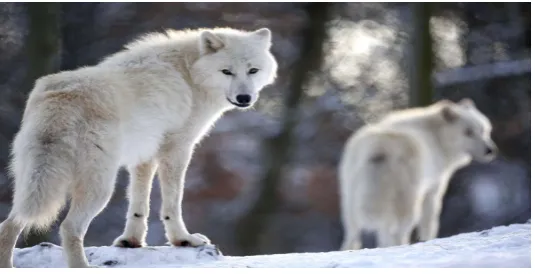
Figure 2.Artic wolves.
The Arctic wolf is also called snow wolf/white wolf orMelville Island wolf. It is the only species to
still be found in their naturally habitats [14]. This does not mean their habitat constants and can be predictable in the future. They hibernate extremely during the long and dark winters. During winter,
temperatures drop as low as -40oC. They are able to survive up to a week without food due to the thick
fur and large bones [7, 8]. The artic wolf is different from other wolves as they live in small family
group. They will roam up to 2600 km2to hunt for food [5]. It is because they are not fast runners and
rely on their stamina to take down prey.
In statistical process control, an early assumption is needed which are the sample observation must be independent and process observation must follow a normal distribution. However, precise data are not always available. In real data, shifted or standard deviation may occur which cause the observation shifted to non-normal distribution [5, 9, 10]. There are other quite considerable studies were carried out to merge statistics with other areas nowadays [11, 12, 13].
2. Materials and Methods
The study used statistical software SPSS 20 and excels 2010 to analyse the data. The demographic characteristics were applied. There are seven independent variable and two dependent variables in the data. The suitable statistical methods to analyse in this study are analysis of variance (ANOVA) and multivariate analysis of variance (MANOVA) [16].
Source of Data Set
Data were taken from http://psych.colorado.edu taken from Skull morphometric data on Rocky Mountain and Arctic wolves (Canis Lupus L, 1990) and (Jolicoeur ,1959:1975). The title of the data is Morphometric data on Rocky Mountain and Arctic Wolves.
Description of Dataset
3
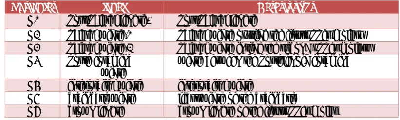
[image:4.595.87.498.186.310.2]variables are post, palatal width-1, palatal width-2, postg foramina width, interorbital width, braincase width and crown length.
Table 1.quantitative variables in Independent variable.
Variables label Descriptions
X1 post palatal length, post palatal length
X2 palatal width-1 palatal width outside the first upper molars
X3 palatal width-2 palatal width inside the second upper molars
X4 postg foramina
width width between the postglenoid foramina
X5 interorbital width interorbital width
X6 braincase width least width of the braincase
X7 crown length crown length of the first upper molar
Table 2.qualitative variables in Independent variable.
Variables Descriptions
Sex 1 = male wolf 2=female wolf
Location 1=rocky mountain 2=arctic
Levene Test for Equality of Variances
Levene's test ( Levene 1960) is used to test ifk samples have equal variances. Equal variances across
samples is called homogeneity of variance. Some statistical tests, for example the analysis of variance, assume that variances are equal across groups or samples [16]. The Levene test can be used to verify that assumption. There are the procedures for levene test:
Step 0: Check the assumptions
Step 1: State the null,H0and alternative hypothesis,H1
Step 2: Decide on the significant level, α
Step 3: Determine the critical value and rejection region
Classical approach P-value approach
Critical value Fα(df = t-1, df2= N-t) N/A
Rejection region FLavene≥ Fα(df = t-1, df2= N-t) p-value≤α
Step 4: Compute Lavene’s Statistic
2 1 ( ) ( 1) n i lavene i i D D F n t
= 2 1 1 ( ) ( ) n n ij ii i D D
N t
(1)Step 5: Make decision
If the value of the test statistic, FLevene, falls in the rejection region or ifp-value ≤ α, then reject H0 ;
otherwise, fail to rejectH0.
Kolmogorov-Smirnov Goodness-of-Fit Test
The Kolmogorov-Smirnov test is used to decide if a sample comes from a population with a specific distribution. The Kolmogorov-Smirnov (K-S) test is based on the empirical distribution function
(ECDF). GivenN ordereddata pointsY1, Y2, ..., YN, the ECDF is defined as [16],
( ) /
N
E n i N (2)
where n(i) is the number of points less than Yi and theYi are ordered from smallest to largest value.
This is a step function that increases by 1/N at the value of each ordered data point. The steps
procedure for Kolmogorov-Smirnov test:
Step 0: H0: The data follow a specified distribution
Ha: The data do not follow the specified distribution
Step 1: The Kolmogorov-Smirnov test statistic is defined as
1
max ( )i i , i ( )i
D F Y F Y
N N
(3)
where F is the theoretical cumulative distribution of the distribution being tested which must be a
continuous distribution. Step 3: Significant level, α Step 4: Critical value
The hypothesis regarding the distributional form is rejected if the test statistic, D, is greater than the
critical value obtained from a table. There are several variations of these tables in the literature that use somewhat different scaling for the K-S test statistic and critical regions. These alternative formulations should be equivalent, but it is necessary to ensure that the test statistic is calculated in a way that is consistent with how the critical values were tabulated.
Shapiro-wilk normality test
The Shapiro–Wilk test is a test of normality in frequents statistics. It is usually used by researcher to check the normality in their analysis [16]. The formula to find the Shapiro-wilk test is:
2
2 1
( ) ( )
i i n
i i
a x W
x x
(4)where
x(i)(with parentheses enclosing the subscript index i) is the ith order statistic
xis the sample mean
aiis the constant
Multivariate Analysis of Variance (MANOVA)
Multivariate analysis of variance (MANOVA) is simply an ANOVA with two or more dependent variables. Moreover, ANOVA tests for the difference in means between two or more groups, while MANOVA tests for the difference in two or more vectors of means. A multivariate analysis of variance (MANOVA) could be used to test this hypothesis [15, 16].
5
3. Results
MANOVA
[image:6.595.106.491.214.465.2] [image:6.595.108.490.217.469.2]MANOVA and some of statistical methods have been applied in this research to fulfil the objectives in this research. The results come out stated as below:
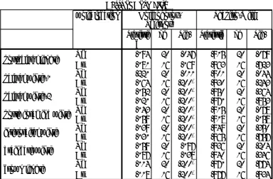
Table 3.Normality test
Tests of Normality
wolf_location
Kolmogorov-Smirnova Shapiro-Wilk
Statisti
c df Sig. Statistic df Sig.
postpalatal length RmAr .194.181 2016 .047.169 .915.963 2016 .079.723
palatal width-1 RmAr .221.164 2016 .200.011* .901.930 2016 .044.243
palatal width-2 RmAr .152.121 20 .20016 .200** .950.971 2016 .364.853
postg foramina width RmAr .143.159 20 .20016 .200** .915.918 2016 .078.158
interorbital width RmAr .139.131 20 .20016 .200** .949.965 2016 .350.757
braincase width RmAr .159.187 2016 .197.138 .936.940 2016 .204.346
crown length Rm .114 20 .200* .971 20 .774
Ar .118 16 .200* .977 16 .934
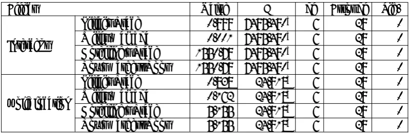
Table 3 above shows the test for normality for all the variables on each group. All thePvalue from the
Shapiro-Wilk statistic are greater than 0.05 thus it can be concluded that all variables are normally distributed.
Table 4.Box's Test of Equality of Covariance Matrices.
Box's M 25.615
F 0.981
df1 21
df2 3801.91
Sig. 0.484
Table 5.Multivariate test.
Effect Value F df Error df Sig.
Intercept
Pillai's Trace 0.999 7495.490b 6 29 0
Wilks' Lambda 0.001 7495.490b 6 29 0
Hotelling's Trace 1550.79 7495.490b 6 29 0
Roy's Largest Root 1550.79 7495.490b 6 29 0
wolf_location
Pillai's Trace 0.838 24.918b 6 29 0
Wilks' Lambda 0.162 24.918b 6 29 0
Hotelling's Trace 5.155 24.918b 6 29 0
Roy's Largest Root 5.155 24.918b 6 29 0
Table 6.Levene's Test of Equality of Error Variances.
F df1 df2 Sig.
postpalatal length 0.132 1 34 0.719
palatal width-2 1.159 1 34 0.289
postg foramina width 0.105 1 34 0.747
interorbital width 2.793 1 34 0.104
braincase width 2.102 1 34 0.156
crown length 1.801 1 34 0.189
The standard Levene's test is a statistical tool to test the assumption of equal variances for each
dependent variables. All six dependent variables showed nonsignificant p value with value greater
than 0.05, so the null hypotheses regarding equal variances can not be rejected for either dependent variable, thus ANOVA are fine (Table 5-6).
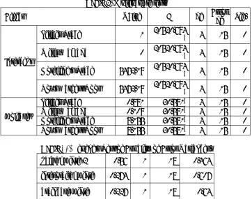
[image:7.595.90.476.490.762.2]Manova for Rocky Mountain (rm)
Table 7.Normality values. wolf_se
x Kolmogorov-Smirnov
a Shapiro-Wilk
Statistic df Sig. Statistic df Sig.
postpalatal length male 0.115 10 .200* 0.974 10 0.925
female 0.2 10 .200* 0.953 10 0.703
palatal width-1 male 0.164 10 .200* 0.873 10 0.109
female 0.154 10 .200* 0.919 10 0.353
palatal width-2 malefemale 0.1750.19 1010 .200.200** 0.9140.956 1010 0.3080.735
postg foramina
width male 0.199 10 .200
* 0.93 10 0.445
female 0.16 10 .200* 0.938 10 0.528
interorbital width malefemale 0.1650.259 1010 0.056.200* 0.9570.892 1010 0.7560.179
braincase width male 0.152 10 .200* 0.917 10 0.331
female 0.214 10 .200* 0.898 10 0.208
crown length male 0.166 10 .200* 0.954 10 0.72
7
[image:8.595.227.368.154.247.2]Table 7 shows the test for normality for all the variables on each group. All the P value > 0.05 in Shapiro-Wilk statistic, thus can be concluded that all variables are normally distributed.
Table 8.Equality covariance.
Box's M 8.445
F 0.637
df1 10
df2 1549
Sig. 0.783
[image:8.595.117.480.349.634.2]An assumption of the MANOVA is that the covariance matrices of the dependent variables are the same across groups (determined by levels of the independent variable) in the population. This assumption is also applied in ANOVA by looking at Box's M tests value (Table 8). The significance value showed to be greater than 0.05 and suggestion have been made. It is suggested that the hypothesis of equal covariance matrices can not be rejected and not violated.
Table 9.Multivariate test.
Effect Value F df Errordf Sig.
Intercept
Pillai's Trace 1 20520.694b 4 15 0
Wilks' Lambda 0 20520.694b 4 15 0
Hotelling's Trace 5472.19 20520.694b 4 15 0
Roy's Largest Root 5472.19 20520.694b 4 15 0
wolf_sex
Pillai's Trace 0.891 30.581b 4 15 0
Wilks' Lambda 0.109 30.581b 4 15 0
Hotelling's Trace 8.155 30.581b 4 15 0
Roy's Largest Root 8.155 30.581b 4 15 0
Table 10.Levene's Test of Equality of Error Variances.
palatal width-2 0.56 1 18 0.464
interorbital width 0.274 1 18 0.607
braincase width 0.227 1 18 0.64
crown length 0.05 1 18 0.825
The test in Table 9 shows there are no significant values with p-value> 0.05. Thus, the (H0 = equal
Manova for Artic (ar)
Table 11.Test of normality.
wolf_sex Kolmogorov-Smirnova Shapiro-Wilk
Statistic df Sig. Statistic Df Sig.
postpalatal
length male 0.198 10 .200
* 0.92 10 0.358
female 0.272 6 0.188 0.878 6 0.259
palatal
width-1 malefemale 0.2640.292 106 0.0470.121 0.8460.765 106 0.0530.028
palatal
width-2 male 0.117 10 .200
* 0.987 10 0.992
female 0.25 6 .200* 0.887 6 0.303
postg foramina width
male 0.212 10 .200* 0.91 10 0.283
female 0.187 6 .200* 0.917 6 0.483
interorbital
width male 0.196 10 .200
* 0.92 10 0.36
female 0.318 6 0.058 0.771 6 0.032
braincase
width male 0.191 10 .200
* 0.931 10 0.46
female 0.269 6 0.2 0.906 6 0.412
crown
length male 0.153 10 .200
* 0.947 10 0.633
female 0.154 6 .200* 0.989 6 0.987
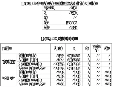
Table 11 shows the test for normality for all the variables according to each group. Most of the theP
[image:9.595.100.479.453.746.2]value from the Shapiro-Wilk statistic are greater than 0.05 except for ‘palatal width-1’, thus it can be concluded that only variable ‘palatal width-1’ for female are non normally distributed.
Table 12.Box's Test of Equality of Covariance Matrices.
Box's M 13.73
F 0.874
df1 10
df2 506.163
Sig. 0.557
Table 13.Multivariate test.
Effect Value F df Errordf Sig.
Intercept
Pillai's Trace 0.999 3653.223b 4 11 0
Wilks' Lambda 0.001 3653.223b 4 11 0
Hotelling's Trace 1328.45 3653.223b 4 11 0
Roy's Largest Root 1328.45 3653.223b 4 11 0
wolf_sex
Pillai's Trace 0.325 1.327b 4 11 0.32
Wilks' Lambda 0.675 1.327b 4 11 0.32
Hotelling's Trace 0.483 1.327b 4 11 0.32
9
The MANOVA above shows that the p-value greater than alpha 0.05, thus we can conclude that the
means vector between male and female for artic wolves are equal (Table 12-13).
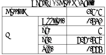
[image:10.595.195.371.184.275.2]Discriminant analysis
Table 14.Box M-Test.
Box's M 3.616
F
Approx. 0.543
df1 6
df2 7271.569
Sig. 0.775
The Box M-Test above (Table 14) tests the null hypothesis of equal population covariance matrices.
Since the p value is greater than alpha (0.05) , the study failed to reject H0. Therefore, it can be
[image:10.595.165.425.344.426.2]concluded that the population covariance matrices are equal for all group.
Table 15.Prior Probabilities for Groups. wolf_location Prior UnweightedCases Used in AnalysisWeighted
rm 0.556 20 20
ar 0.444 16 16
Total 1 36 36
[image:10.595.140.430.489.623.2]Table 15 shows the prior probabilities for groups for wolve rocky mountion is 0.556 and for arctic is 0.444. The prior probability is unequal since the number of observation for RM wolves and AR wolves are not equal.
Table 16.Classification results.
wolf_location
Predicted Group
Membership Total
rm ar
Original
Count rm 20 0 20
ar 1 15 16
% rm 100 0 100
ar 6.3 93.8 100
* 97.2% of original grouped cases correctly classified.
Table 16 shows the confussion matrix of group predicted. All cases for Rocky Mountain wolves are correctly predicted. On the other hand, one Arctic wolf is misclasified into Rocky Mountain’s group. Thus the total perfomance for the discrminant function analysis is 97.2% correct.
4. Conclusions and Discussions
Further research recommended increasing the precision in RM wolves and artic wolves by using another statistical model or method such as fisher linear discriminant function and exploratory factor analysis.
Acknowledgement
The research work is supported by FRGS (Fundamental Research Grant Scheme) grant (vot 1498), Ministry of Higher Education, Malaysia.
References
[1] Adams D C and Erik O-C 2013 Geomorph: An R Package For The Collection And Analysis Of
Geometric Morphometric Shape DataMethods in Ecology and Evolution393-399
[2] Fred C L, Scott E H and Charles J J 1994 Prevention And Control Of Wildlife Damage
Cooperative Extension Division Institute of Agriculture and Natural Resources (University of Nebraska – Lincoln)
[3] Faulkner J 1987 Northern Rocky Mountain Wolf Recovery PlanU.S, Fish and Wildlife Service
in cooperation with the Northern Rocky Mountain Wolf Recovery Team119
[4] Klingenberg and Peter C 2011 Morphoj : An Integrated Software Package For Geometric
MorphometricsMolecular Ecology Resources353-357
[5] Lakshmi D and Yellamma K 2013 The Promontory Role Of Trace Element And Nutrients On
Morphometric Traits In The SilkwormBombyx mori Int. J. Pure App. Biosci 11-18
[6] Petersen M 2011 Insular And Disjunct Distribution Of The Arctic Wolf In Greenland Polar
Biology1447–1454
[7] Petersen M 2012 Decline And Extermination Of An Arctic Wolf Population In East Greenland
Arctic65(2) 155-186
[8] David M 2015 Annual Arctic Wolf Pack Size Related to Arctic Hare NumbersArctic 60(3)
300-311
[9] Bin Shafi M A, Bin Rusiman M S and Che Yusof N S H 2014 Determinants Status of Patient
After Receiving Treatment at Intensive Care Unit: A Case Study in Johor Bahru.I4CT 2014
- 1st International Conference on Computer, Communications, and Control Technology, Proceedings 30 September 2014, 6914150 80 – 82
[10] Shafi M A and Rusiman M S 2015 The Use of Fuzzy Linear Regression Models for Tumor Size
in Colorectal Cancer in Hospital Of MalaysiaApplied Mathematical Sciences 9 (56)
2749-2759.
[11] Rusiman M S, Nasibov E and Adnan R 2011 The Optimal Fuzzy C-regression Models
(OFCRM) in Miles per Gallon of Cars Prediction, Proceedings – 2011 IEEE Student
Conference on Research and Development, SCOReD 2011, 6148760 333-338
[12] Rusiman M S, Hau O C, Abdullah A W, Sufahani S F, Azmi N A 2017 An Analysis of Time
Series for the Prediction of Barramundi (Ikan Siakap) Price in MalaysiaFar East Journal of
Mathematical Sciences102(9) 2081-2093
[13] Nor M E, Rusiman M S, Mohamad N A I and Lee M H 2017 Directional Change Error
Evaluation in Time Series ForecastingAIP Conference Proceedings1830 (1) 080013
[14] Siminski D P 2000 Mexican Wolf SSP Annual Meeting And Reunion Binacional Sobre El Lobo Mexicano (Arizona-Sonora Desert Museum Tucson, Arizona)
[15] Awang Z 2010 Research Methodology for Business and Social Science Malaysia (Universiti
Teknologi Mara Publication Centre (UPENA) )
[16] Awang Z 2012 Research Methodology and Data Analysis 2nd ed Selangor(Dee Sega