AUTOMATIC SPOKEN LANGUAGE RECOGNITION FOR MULTILINGUAL SPEECH RESOURCES

8183

1_{ASMA SBAI,} 2 _{ABDELALI TOUIL and} 3 _{FATTEHALLAH GHADI}

1, 2, 3 _{Laboratory of Engineering Science, Faculty of Science, Ibn Zohr University, Morocco}

E-mail: 1_{[email protected],} 2_{[email protected],} 3_{[email protected]}

ABSTRACT

Previous studies had investigated the estimation of demand using either static or dynamic approach. Each approach has its positive and negative side. During these last years, more attention was given to the combination of static and dynamic models and the integration of traffic assignment to obtain a more accurate updated matrix. In this paper, we present a simulation where we use the entropy-based gravity model to generate a seed matrix then we update the links costs using Stochastic User Equilibrium assignment model to obtain a new estimation. We show that incorporating an assignment method to the process of estimation of Origin Destination Matrix lead to a better estimation.

Keywords: Dynamic gravity models; Transport planning; Origin Destination Matrix; Gravity model; Stochastic User Equilibrium

1. INTRODUCTION

Managing the economic development, satisfying the demand of citizen for uncongested transportation network and protecting the environment and citizen wellbeing are all a huge concern of city managers. Thus, one of the fundamentals of a smart city is to create an environment of intelligent devices and an efficient network that support digital applications for decision making of urban planners and designers. Relaying on technology, both hardware and software, it is more feasible than before to collect and analyze rich datasets and consequently improve the management of traffic and forecast of urban flows which lead to an intelligent management of the city. This raise advanced applications within a discipline named Intelligent Transportation System (ITS). It aims to provide innovative services related to traffic management to inform users and help them make safer and smarter use of transport network. Developing such optimal system is a challenging problem as transportation networks are often large with infinite constraints. All of this can’t be done without mathematical models which are a simplified representation of complex problem. Thus, the added value of advanced processing of datasets and dynamic traffic models is offering as maximum as possible real time information about the instant state of the transportation network.

One of the most important inputs to traffic simulation models is the Origin-Destination Matrix

(ODM). It is one of the most challenging obstacles to overcome before deploying traffic modeling for planning application. Usually, ODM were estimated through home and roadside interviews, license plate surveys, etc. Those methods are expensive to conduct and also incapable of estimating real-time ODM.

To achieve trip distribution studies in the most accurate way, we may rely on prior information about the network. So we work with historical data or on user demand and demographic information based on earlier surveys or historical data. We can also retrieve data from different sensors, cell phones, mobile apps or using automated vehicles or in-cars devices. Then this data is processed to create a predicted ODM that is used as an input to design or monitor an urban network. Recently, more researchers are interested in combining different approach to achieve better results regarding estimation of the ODM. One of the most interesting combinations is iterating between static methods of traffic distribution and dynamic assignment.

Thus in this paper, we will discuss the efficiency of using entropy-based gravity model for dynamic trip distribution purpose and iterated it with a dynamic assignment method: Stochastic User Equilibrium (SUE) approach for updating cost of

ISSN: 1992-8645 www.jatit.org E-ISSN: 1817-3195

8184 each path. Plus we will investigate the use of two different deterrence functions and the impact of the choice of this function on the estimation process. The paper is organized into six sections. After the introduction, the second section is dedicated for the four step model, a framework of transportation systems. Section 3 presents the state of the art and the most important works about trip distribution and traffic assignment. Section 4, describes the problem formulation. Section 5; provides experimental results, and finally a conclusion.

2. FRAMEWORK OF TRANSPORTATION SYSTEM

Transportation planners are engaged in the following issues of mobility: congestion, land use, protection of environment, financing, equity and special need travelers. Thus they are concerned by the following tasks: estimation of future demand, making an evaluation of the current network configuration, proposing an upgrade by making facilities available by different services, calculating the cost of mobility, studying the options and making solutions available in time. Accordingly, travel frameworks are used to provide objectively the advantages and disadvantages of each alternative, which consist on change of policies, network configuration, socio-economic possibilities, demographic evolution or any other influential factor. One of the primary tools for forecasting future demand and evaluating the performance of transportation system is the four step model, which have evolved over many decades.

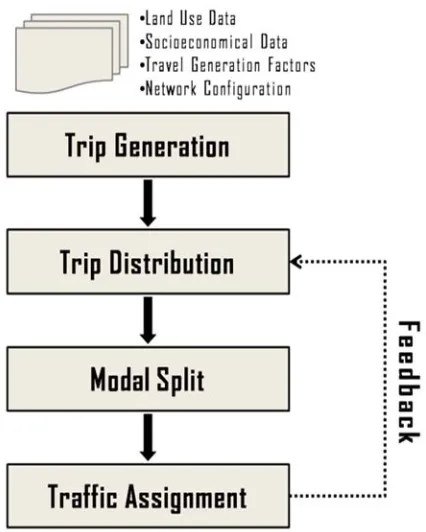
Introduced in the 50’s[1], this framework is widely used to support transportation projects and consider the trip the unit of analysis. As its name referred, the first step is trip generation, which defines the number of trips produced and attracted by zone. In the second step, trip distribution, trips are distributed in a two dimensional table that represent the number of demand from an origin to a destination. Then in the third step, modal choice, trip tables are split to different trip tables by transportation mode (passenger, automobile, bicycle…etc) considering travel time or distance. In the last step, traffic assignment, the process of assigning the traffic demand to the routes on a road network. The trips are assigned considering that the users want to minimize their travel time or are moving in the existing state of the network: If the

traffic exceeds the capacity of the segments congestion occurs and negatively affects the traffic, which through a feedback process influences trip distribution.

Figure 1 Four Step Model Of Transportation Framework

3. STATE OF THE ART AND RELATED WORK

3.1 The Origin Destination Matrix Estimation

8185 as its name refer, depends on time and the produced matrix is for short-term planning such as route guidance or traffic control. According to [3] various approaches may also be categorized by prior hypothesis on nature of traffic: route choice proportions, travel time, travel time dispersion, data sources: observation from probe vehicles, license plate readers or the estimation techniques: Least squares, maximum likelihood or Kalman filtering.

Static approaches are the most commonly used, it consists on considering independent time traffic flows to estimate an average OD demand that represent the distribution of the number of vehicles in the network for that time interval. Many researchers have proposed different algorithms for static estimation, such as Casey [4] where he applied the gravity model to find the optimal OD demand. Other approaches first investigated the estimation of ODM in a static network are minimum information, maximum entropy [5]; maximum likelihood [6], [7]: the authors used available trip data such as traffic counts to obtain an ODM. In parallel, others proposed statistical methods where the most known and discussed are Generalized Least Squares [8] and Bayesian approach [9].

In one hand dynamic ODM estimation estimate OD flows based on collected traffic data and are classified in non-assignment based and assignment based models. The non assignment models used inbound and outbound traffic volumes based on the law of traffic volume conservation, but those methods do not take into consideration microscopic behaviors such as signal delays. In the other hand, the assignment-based methods are performing more accurately the estimation by relaying on dynamic traffic assignment models. As stated by [10], we can also split the assignment base models into five sub-categories: the generalized least square models, bi-level models, Bayesians approach, maximum entropy models and state space models. The dynamic methods are designed for short-term traffic purposes, so researchers such as [11] designed algorithms that rely on the link volume and traffic conditions, [12] has used the Bayesian inference to update a prior OD matrix using time-varying traffic counts. Additionally, researchers were interested in applying the Kalman filtering technique to estimate dynamic O–D matrices [13] [14] [15] [16].

Dynamic OD estimation is more complex than the static one, because a time index is required and thus the algorithms are consuming more time and resources proportionally to the size of the network. On the contrary, static models are simple to implement and need less time to compute but those models’ output is an average OD demand per interval of time and thus is not giving explicit information about real-time state of the system.

3.2 The Entropy Based Gravity Model Formulation

Gravity model is a widely used model in different disciplines (such as: physics, trade and transport) and has its origins from the Newton law. Based on its application, [17] has proposed a formulation of gravity model. This study assumes that the traffic from a zone origin i to a zone

destination j: T is related to network features and

to the land proportion using the following equation:

T

Where P is the population in the zone

and P is the population of zone and d is the

distance between the two zones.

Wilson [18] assumes that the interaction between two sites declines with increasing distance, cost and time of travel but is positively correlated with the amount of activity at each site. The proposed model is then known as the doubly constrained gravity model so that total trips from zone i and total trips to zone j are equal to total origins and destination respectively. The equation (2) represents the formulation as introduced by [18], which is a generalization of the doubly constraint gravity model with a negative exponential cost function. It’s also a result from entropy maximization approach.

T A O B D e (2)

A

∑ (3)

B

ISSN: 1992-8645 www.jatit.org E-ISSN: 1817-3195

8186

T Total number of trips

T Number of trips modeled from zone

origin i to zone destination j

O Trip produced from zone i

D Trips attracted to zone j

C Distance between zone i and zone j

f Deterrence function

A , B Coefficient that are set to meet the margin constraints of the Origin Destination Matrix

t Number of trips observed from zone

origin i to zone destination j

n Number of zones

To obtain equation 2, [18] considered that

the probability of distribution of T happening is

proportional to the number of states of the system which imply this distribution, and satisfy the following constraints:

∑ T O (5)

∑ T D 6

∑ T C, C 7

T ∑ O ∑ D 8

Using the entropy maximization, we found that the most probable distribution of trips is expressed in the same way as the gravity distribution equation, and thus constitute a theoretical base for the gravity model. Still, the parameter β in the negative exponential function need to be calculated using a calibration process.

3.3 Extension to Dynamic Distribution

In 1990, [19] was the first authors that provided the formulation of the dynamic extension of the gravity model, the proposed model was intended for prediction of trip demand in relation with past distribution and updated travel cost. Based on this work, several gravity-based models

have been investigated based on surveys or traffic counts data such in the works of [20] and [21].

In 2006, comes [22] with a doubly dynamic gravity model (DDGM) that takes into accounts inter-period and intra-period evolution of travel demand as function of travel cost. They incorporate traffic assignment into the procedure and a time-series of traffic counts.

In 2011, [23] investigate the use of a dynamic time-dependent gravity model with a revised impedance function for evacuation purposes in the case of a hurricane. The approach was developed based on static model but was extended to be sensitive to network conditions, available

accommodation and path prediction. The

impedance function used was a combination between negative exponential and Rayleigh functions.

In 2017, authors in [24] estimates a dynamic OD distribution by first creating a static ODM starting from a static model using the QUEENSOD and then via the software INTEGRATION where this data is considered as an input also called a seed matrix to adjust through time slices and generate a dynamic OD matrix.

3.4 Traffic Assignment

The traffic assignment consists on the allocation of trip interchanges to a specific transport network. To do that, we need a detailed description of the transportation system and a matrix of inter-zonal movements. The output is principally the estimation of traffic volumes and corresponding costs on each link of the system, some sophisticated model includes directional turning movement at intersections and route flows.

One of the main purposes of the traffic assignment is to evaluate the deficiencies in the existing system by assigning estimated future trips to the existing system and test alternative transportation system proposals. The early studies (1940’s) consisted on estimating the diversion of traffic from existing road to new improved ones for two purposes: saving travel time and cost.

8187 were independent of the flows. The results amounted to the proposed road being used either by all vehicles between a pair of OD or by no vehicle, which is unrealistic. Experimental studies were later trying to join the choice of route to time and distance factors. The American Association of State Highway and Transportation Officials (AASHTO) develop a standard diversion curve. Those curves are obtained from the observation on similar locations and estimate the proportion of flow to be redirected to the new links. Different formulas where developed generally depending on travel cost and assume that travel time is independent of volume of traffic on links and therefore does not take time congestion in consideration. This technique is known as proportional assignment. In early 1950’s, researches introduce the user’s road choice in consideration. The difficulty was that the route choice was arbitrary and depends on the engineer personal perspective and experience and the travel time, cost and distance. The 1957 brings-in the shortest route method which became the main component for the traffic assignment problem. The researchers used the Moore’s method to develop a program to find the shortest route based on the average link travel time and speed. The result was the barely improvement of all-or-nothing assignment since all the users are redirected to the cheapest route and is easy to program in one step with no iteration but lead to the quiet same unrealistic results given that all traffic is assign to the chosen route with limited capacities and lead automatically to congestion. In 1952, [25] published a research on the two principals of flow distribution:

 The user equilibrium principal: “All

travelers are minimizing their own travel cost”.

 The system optimum principal: “Travelers

choose their route as to minimize all the system travel cost”.

Improved assignment techniques were investigated taking into consideration the two principals of Wardrop, and new algorithms immerge where travel time was recalculated iteratively taking into consideration the congestion effect. So a need for equations that bound the travel time, speed and cost to the traffic volume on links were developed which are known as link performance function.

Different laboratory developed their link performance formula. In general the formulas were presented according to the observation on network characteristic, travel time and speed. The basic parameters are:

 The free flow travel time: The measure of

travel time at zero flow

 The practical capacity: The volume from

where the travel time starts to increase if the volume flow continues on amplifying.

4. PROBLEM FORMULATION 4.1 Stochastic User Equilibrium (SUE)

Introduced by Daganzo and Sheffi in 1977 [26] then by Fisk in 1980 [27], Stochastic User Equilibrium SUE aims to combine stochastic assignment with Wardrop Equilibrium to rise above the limitation of homogeneous user assumption in Wardrop equilibrium and to take into consideration the random effect of stochastic assignment problem. SUE is then used to analyze a network taking in consideration an ODM to find the flows in all the links of the considered case. This class of methods also called multipath assignment; aims to model the change in driver perceptions and allow the drivers to choose routes based on their knowledge. Thus, SUE assumes that the drivers do not have a complete knowledge of the network conditions, which make it a more realistic assumption. This is translated by assigning trips probabilities – which represent the likelihood of using a particular link to travel from an origin to a destination – to alternative paths, so multiple paths, are considered in the assignment process.

4.2 Cost Functions

For the exponential cost function, only one parameter β needs to be calibrated and is widely used in research and case study. The equation is meant to reproduce the effect of distance and cost of mobility between two zones. So people behavior is such the further or the more expensive the destination, the less frequently they move there.

ISSN: 1992-8645 www.jatit.org E-ISSN: 1817-3195

8188

f C e β ₉

In 1961[28], authors combines the exponential and the power functions to obtain the following equation called tanner cost function. In this case the distribution modeled is constrained to reproduce the means of both cost and its logarithms (eq 13, eq14)

f C Cα_{. e} β ₁₀

To find the parameters of the cost function, a calibration process is needed. We apply the maximum likelihood approach to reproduce distribution from initial observation [29] respecting the following equations and using the Hyman [30] approach of variable neighborhood search. It has been proved to be one of the fastest and simplest methods.

∑ T O 11

∑ T D 12

∑ C T ∑ C t 13

∑ log C T ∑ log C t 14

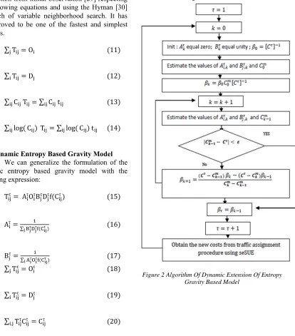
4.3 Dynamic Entropy Based Gravity Model

We can generalize the formulation of the dynamic entropy based gravity model with the following expression:

Tτ _Aτ_Oτ_Bτ_Dτ_{f C}τ ₁₅

Aτ

∑ τ τ τ 16

Bτ

∑ τ τ τ 17

∑ Tτ _Oτ ₁₈

∑ Tτ _Dτ ₁₉

∑ Tτ_Cτ _Cτ

, 20

Tτ _{∑ O}τ _{∑ D}τ ₂₁

τ corresponds to starting time of a slice of time of a global study interval. The generalized cost

for period τ used in this formula C is the result of

SUE traffic assignment method.

The following figure 2 represents the steps of the procedure of estimating the ODM using the dynamic entropy based gravity model.

We denote: C the observed Mean cost

from observed traffic length distribution at slice

interval τ. Where C Modeled Mean cost from

modeled traffic length distribution at iteration k

8189

5. EXPERIMENTAL RESULTS

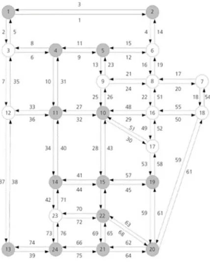
The experiments were conducted on the Sioux fall network, a wildly used test network in the literature. It’s composed of 24 nodes, 76 links and 576 OD pairs [31].

Figure 3 Sioux Fall Network Simplified Graph

We performed the experiments on seSUE an open source software [32] using .Net Framework 4.5 and the method of Stochastic User Equilibrium SUE, which is a relaxation of Wardrop User Equilibrium principals. This software is developed by: Selin Damla Ahipaşaoğlu,Uğur Arıkan, and Karthik Natarajan at the Engineering Systems and Design (ESD) pillar in Singapore University of Technology and Design (SUTD). We will combine seSue with a Matlab implementation of dynamic entropy based gravity model, using Matlab R2014a under a 32-bit machine.

To measure the performance of the algorithm we used the Root Mean Square Error (RMSE), Standardize Root Mean Square Error (SRMSE) and the correlation (r²) between observed and synthesized matrices.

RMSE ∑ ² 22

SRMSE

∑ ² ∑

²

23

Figure 4 Structure Of Code Implementing The Tests

ISSN: 1992-8645 www.jatit.org E-ISSN: 1817-3195

8190

5.1 Results From Case 1:

The first case we investigate was the use of exponential deterrence function (eq 9) with one parameter to calibrate.

Table 1 Results of the experiments on Exponential function (eq 9)

Exponential Cost Function

Interval β r² RMSE SRMSE

1 -0.1228 0.746 14.51 0.5565

2 -0.0307 0.749 14.43 0.0231

3 -0.0387 0.760 14.12 0.0226

4 -0.0383 0.761 14.10 0.0225

We can observe from the first test using the exponential function that there is a significant amelioration of the RMSE and the SRMSE as the number of iterations increase.

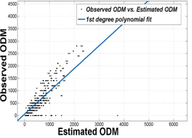
Figure 5 Fit Evaluation Of Observed Vs Estimated ODM: Case Of Exponential Deterrence Function

Figure 6 Fit Evaluation-Residuals For The Observed Vs Estimated ODM: Case Of Exponential Deterrence

Function

From figure 5 and figure 6 we can also deduce that the model is correct since our approach reproduced almost 80% of the observed ODM.

5.2 Results from Case 2:

The second case experimented is the tanner deterrence function (eq10) with two parameters to calibrate.

Table 2 Results Of the Experiments On Tanner Deterrence Function (eq 10)

Tanner Cost Function

Interval α β r² RMSE SRMSE

1 -0.12 +0.18 0.654 16.99 0.027

2 -0.18 -0.035 0.740 16.59 0.026

3 -0.028 -0.025 0.763 14.04 0.022

4 -0.12 -0.030 0.772 13.93 0.022

In this case too, in table 2 we can observe the evolution of RMSE and SRMSE toward better values and so less error.

8191

Figure 8 Fit Evaluation-Residuals For The Observed Vs Estimated ODM: Case Of Tanner Deterrence Function

The conducted fit evaluation in figure 7 and figure 8 shows that our approach is also valid in the case of using tanner deterrence function.

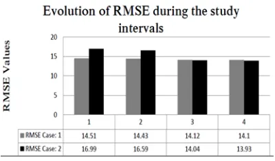
Figure 9 Evolution Of RMSE During The Study Interval For Both Cases

The RMSE graph Figure 9 shows that although tanner deterrence function show more errors but in the end achieves a slightly better estimation than the exponential function.

However, the additional term added to the exponential deterrence function to create the tanner function, didn’t add much to the model, so we can omit it and use only the exponential function especially that it present an acceptable RMSE from the first iteration.

6. CONCLUSION

Many investigators have study the multi-level approach for estimation of ODM but the impact of deterrence function and the choice of these parameters were not always taking into

consideration. This paper investigated the estimation of ODM by extending the gravity model to dynamic approach by the use of Stochastic User Equilibrium assignment model and two different cost functions. In one hand, we can observe a small change in the structure of the dynamic ODM depending on the choice of the deterrence function. In this case study, the use of exponential deterrence function is sufficient and using tanner function will just add to the complexity of the problem, since the improvement observed was not major. I the other hand, the dynamic approach was represented by the adjustment of Origin Destination Matrix into current traffic condition based on stochastic user equilibrium method for dynamic assignment and time series of link travel costs.

Although we have studied the evolution of Origin Destination Matrix across successive intervals of global study period, dynamic extension of entropy based gravity model can be used for the prediction of future demand and the forecast of path costs.

For future work, we will try to find a way to take in consideration other factors than the route choice parameter to improve the estimation accuracy.

REFERENCES

[1] Ortuzar, J.D., Willumsen, L.G., 1991.

Flexible long range planning using low cost information. Transportation 18, 151–173.

[2] Simonelli F., V. Marzano, A. Papola, I.

Vitiello (2012). A network sensor location procedure accounting for o-d matrix

estimate variability. Transportation

Research part B, vol. 46, p. 1624-1638.

[3] Van Der Zijpp, Nanne. "Dynamic

origin-destination matrix estimation from traffic counts and automated vehicle identification data." Transportation Research Record: Journal of the Transportation Research Board 1607 (1997): 87-94.

[4] Casey, H. 1955. “Applications to Traffic

Engineering of the Law of Retail Gravitation.” Traffic Quarterly 9 (1): 23– 35.

[5] Van Zuylen, H.J. and L. G. Willumsen,

ISSN: 1992-8645 www.jatit.org E-ISSN: 1817-3195

8192 Part B: Methodological, vol. 14, pp. 281-293, 1980.

[6] Bell, M.G.H. (1983). The estimation of

origin-destination matrix from traffic counts. Transportation Science 10, 198-217.

[7] Cascetta, E. and S. Nguyen (1988). A

unified framework for estimating or updating origin/destination matrices from traffic counts. Transportation Research 22B, 437–455.

[8] Cascetta, E. (1984). Estimation of trip

matrices from traffic counts and survey data: a generalized least squares estimator. Transportation Research 18B, 289–299.

[9] Maher, M. (1983). Inferences on trip

matrices from observations on link volumes: a Bayesian statistical approach. Transportation Research 20B, 435–447.

[10]Lu, Zhenbo, et al. "A Kalman filter

approach to dynamic OD flow estimation for urban road networks using multi-sensor data." Journal of Advanced Transportation 49.2 (2015): 210-227.

[11]Djukic, T., J. Barceló Bugeda, M. Bullejos,

L. Montero Mercadé, E. Cipriani, H. van

Lint, and S. Hoogendoorn. 2015.

“Advanced Traffic Data for Dynamic OD Demand Estimation: The State of the Art

and Benchmark Study.” In 94th

Transportation Research Board Annual Meeting, 1–16. Washington, DC: National Research Council.

[12]Cremer, M., and H. Keller. 1987. “A New

Class of Dynamic Methods for the

Identification of Origin–Destination

Flows.” Transportation Research Part B 21 (2): 117–132.

[13]Ashok, K., and M. E. Ben-Akiva. 2000.

“Alternative Approaches for Real-time Estimation and Prediction of Time-dependent Origin–Destination Flows.” Transportation Science 34 (1): 21–36.

[14]Soule, A., K. Salamatian, A. Nucci, and N.

Taft. 2005. “Traffic Matrix Tracking Using

Kalman Filters.”ACMSIGMETRICS

Performance Evaluation Review 33 (3): 24–31.

[15]Barceló Bugeda, J., L. Montero Mercadé,

M. Bullejos, O. Serch, and C. Carmona. 2012. “A Kalman Filter Approach for the Estimation of Time Dependent OD Matrices Exploiting Bluetooth Traffic Data

Collection.” In 91st Transportation

Research Board Annual Meeting, 1–16. Washington, DC: National Research Council.

[16]Ying, L., J. Zhu, W. Huiyan, and L.

Zhenyu. 2016. “A Novel Method for Estimation of Dynamic OD Flow.” Procedia Engineering 137: 94–102.

[17]Casey, H.J., 1955. Applications to traffic

engineering of the law of retail gravitation. Traffic Quarterly IX (1), 23–35.

[18]Wilson, Alan Geoffrey. "Inter-regional

Commodity Flows: Entropy Maximizing

Approaches." Geographical analysis 2.3

(1970): 255-282.

[19]Dendrinos, D.S., Sonis, M., 1990. Chaos

and Socio-Spatial Dynamics. Springer-Verlag, New York.

[20]Tune, Paul, and Matthew Roughan.

"Controlled Synthesis of Traffic

Matrices." IEEE/ACM Transactions on Networking (2017).

[21]Cascetta, E., Russo, F., 1997. Calibrating

aggregate travel demand model with traffic

counts: Estimators and statistical

performance. Transportation 24, 271–293.

[22]Tsekeris, Theodore, and Antony

Stathopoulos. "Gravity models for dynamic transport planning: Development and implementation in urban networks." Journal of Transport Geography 14.2 (2006): 152-160.

[23]Cheng, Guangxiang, Chester Wilmot, and

Earl Baker. "Dynamic gravity model for

hurricane evacuation planning."

Transportation Research Record: Journal of the transportation Research Board 2234 (2011): 125-134.

[24]Hao Yang & Hesham Rakha (2017): A

novel approach for estimation of dynamic from static origin–destination matrices, Transportation Letters

[25]Wardrop, John Glen. "Some theoretical

aspects of road traffic research." Inst Civil Engineers Proc London/UK/. 1952.

[26]Daganzo, C.F., She , Y., 1977. On

stochastic models of traffic assignment. Transportation Science 11, 253±274

[27]Fisk, C., 1980. Some developments in

equilibrium traffic assignment.

Transportation Research B 14, 243±255

[28]Tanner, JC (1961) Factors affecting the

8193 paper 51. London: Her Majesty’s Stationery Office.

[29]Sbai, A., & Ghadi, F. (2017, October).

Impact of Aggregation and Deterrence Function Choice on the Parameters of Gravity Model. In Proceedings of the Mediterranean Symposium on Smart City Applications (pp. 54-66). Springer, Cham.

[30]Hyman, G. M. (1969). The calibration of

trip distribution models. Environment and Planning A, 1(1), 105-112.

[31]http://www.bgu.ac.il/bargera/tntp

[32]http://people.sutd.edu.sg/ugur_arikan/seSue

[33]Yang, Hao, and Hesham Rakha. "A novel

approach for estimation of dynamic from

static origin–destination

matrices." Transportation Letters (2017): 1-10.

[34]Erlander, S., Stewart, N.F., 1990. The

Gravity Model in Transportation Analysis: Theory and Extensions. VSP, Utrecht.

[35]Boyce, D.E., Janson, B.N. and Eash, R.W.