Journal of Theoretical and Applied Information Technology 30th April 2017. Vol.95. No 8
© 2005 – ongoing JATIT & LLS
ISSN: 1992-8645 www.jatit.org E-ISSN: 1817-3195
ASSESSING LEARNING PARADIGMS IN TEXT
CLASSIFICATION
1MOHAMMED ABDUL WAJEED, MOHAMMAD ABDUL RAHMAN
1
Professor, CSE Keshav Memorial Institute of Technology, Hyderabad, India,
2
Assistant Professor, CSE Keshav Memorial Institute of Technology, Hyderabad, India E-mail: [email protected] , [email protected]
ABSTRACT
Today abundant information is available due to the advent of Internet, which is usually stored with sole purpose of current needs alone. Such data thus rest in unclassified in dump repository. Instead if it would be stored in a classified repository then navigation could be done easily, or classified at the later stage reaching it could become easier and thus could helpful in decision making. In the process of classification, commonly supervised and unsupervised paradigm is adopted. Semi-supervised is a new term which is in-between supervised and unsupervised learning where in-addition to the unlabeled data, the algorithm is provided with some supervision information but not necessarily for all example data. A blend of supervised and unsupervised classification is explored in the formation of fuzzy clusters based on the importance of the terms in each class. Enhancements in traditional KNN algorithm is explored taking into consideration the different weights for the features based on the concept of variance in each class. Finally the results obtained in supervised paradigm and semi-supervised paradigm is compared.
Keywords: Text Classification, Semi-Supervised, Fuzzy-Clusters, Variance, Enhanced-KNN.
1. INTRODUCTION
Man is leading his life today with numerous electronic gadgets for a comfortable life. These gadgets generate bulk data with the sole purpose of proof checking alone. The generated data is stored earlier in unclassified, dump repository. In case if the dump repository could be turned into a classified repository then, future data navigation becomes easier [4]. The classified repository could be useful in future decision making. In the process of data classification much work is already conceded in cases where the data is in a structured format i.e. in the form of rows and columns in the databases, and also some work addressed the progress in classifying the semi-structured data, which exists in the form of HTML files. But not much work is explored relatively in the case of data existing in unstructured format i.e, in raw format, free flow textual form. The paper attempts in classifying the unstructured data using the bag-of-words approach termed as textual classification as in [40] rather than parts-of-speech approach as in [41]
There are usually two approaches in the process of data classification, the supervised and unsupervised approach. In case of supervised approach training data is given, which contains a set of independent attributes along with their
corresponding dependent attribute value which can also called as class label [1] [20]. Using the training data a classifier is trained, built which is subjected to the test data at the later stage. The test data also has the set of independent attributes along with their corresponding class label value. But the class label value is hidden. The classifier built classifies the test data by giving the expected class label which is compared with the actual, thus the classifiers accuracy is obtained. On the other hand in case of unsupervised classification where no such a training data is provided, the given data is stored in clusters in such a way that the intra-similarity within the clusters is maximized and inter-similarity among the clusters is minimized. All the elements belonging to the same cluster are expected to have same class label.
which exists in abundance, is provided to the classifier. The semi-supervised learning algorithm is provided with some supervision information but not necessarily for all data. With a very limited training data a classifier is built which is termed as primary classifier. The primary classifier is subjected to the test data, the class label obtained from the primary classifier is now added to the existing training data, treating it as an additional training data, and a new classifier is built which is expected to be superficial than the primary classifier built earlier, and is termed as next primary classifier. The whole process is repeated to obtain the final classifier which is deemed to be better than all the classifiers built so far. The final classifier is deemed to be superficial in accuracy as it was build using larger training data.
Huge dimensionality, which can also be termed as large number of feature handling, is involved in the process of text classification which is a nightmare. Many supervised and unsupervised techniques already exist in the process of reducing the features. In the present paper an attempt to group the features into clusters based on the importance of the terms in different classes is made. Features in text classification are the terms that occur in the documents. In the process of formation of clusters, Gaussian function is employed due to its superiority over other functions in performance and to have a better quality of clusters formed [29] [30].
The major step in building a classifier is to choose the learning mechanism; in the current paper lazy learner algorithm called K-Nearest Neighbour is adapted, with some enhancements. All features may not be important in all the classes, some features may play vital role in some classes and in others they may have no impact at all. But in traditional KNN algorithm all features are given same importance in all classes which is not reasonable. Taking into consideration the difference in feature importance in different classes, enhancements are made to traditional KNN algorithm [12]. The concept of variance is applied for features in different classes, based on which the weights to the features are assigned differently thus resulting in enhancements. The objective of the study made in the present paper is to compare the classification accuracy in supervised and semi-supervised learning module. The impact of small number of training data in the process of textual data classification is explored.
The paper is organized as follows. In section 2 lexicon generation, training data, test data nomenclature used in the paper are provided. we
outline basic concepts, related background, definitions, and existing techniques in the process of feature reduction techniques are furnished. Although present paper does not employ feature reduction, for the convenience of prospect researchers who may explore, it is provided. The terms used in the data processing are also defined in this section. In section 3 supervised and semi-supervised learning mechanism in text classification using fuzzy clusters with enhancements in KNN algorithm is discussed. In section 4 implementation details of both the supervised and semi-supervised techniques are provided and finally in section 5 results obtained in both the learning mechanism are compared and conclusions are provided.
2. BASIC CONCEPTS AND DEFINITIONS
The key technology for making sense of the high dimensional data is Feature Selection (FS), which is the next major step after the choice of learning mechanism in the process of data classification.
Many FS techniques already exist in the literature [2] [3] [9]. Curse of dimensionality is a major challenge in text classification, in terms of computation efforts and in terms of algorithm implementation in addition to other difficulties. FS primary requirement is to select and separate the relevant informative feature for the classifier from the available large features. In addition FS has got other motives like general data reduction which would limit the storage requirements resulting in increase in algorithm functionality and speed [24] [17]. The next important motive includes the
selection in supervised learning. Techniques like document frequency, term frequency, and inverse-document frequency are consi dered as feature selection in unsupervised learning as they do not take consideration the value of the decision attributes.
Information gain [18] is a supervised feature reduction technique. Given a set of categories Cm,
where m is the number of classes the information gain of term ‘t’ is given by
log (
( ) ( ) log ( ) ( ) ( | )
1 1
| ) ( ) ( | ) log ( | )
1
i i i
i i i
P
m m
IG t P c P c P t P c t
i i
m
c t P t P c t P c t
i
= −∑ + ∑
= =
+ ∑
=
(1)
Chi-Square is another supervised feature selection technique for feature reduction which is given by
2 ( , ) ( , ) ( , ) ( , )
.
( ) ( ) ( ) ( )
k i k i k i k i
k k i i
P t c P t c P t c P t c
N
P t P t P c P c
χ
−−
=
(2)Odds Ratio is yet another supervised feature selection method which is given by
( | ). ( | )
(1 ( | )). ( | )
k i k k
k i k k
O R P t c P t c
P t c P t c
=
− (3)
Based on the values obtained in the above equations, which determines the relationship between the terms and the class label, feature selection can be made.
Definitions: - We are provided with the training
document set Ts whose class label is given along
with the document. We are also given a set of document set Tt termed as test data set whose class
label is to be determined by the classifier. Lexicon set £ is a set which contains all words, that have appeared in the training document set Ts.
We find the patterns of each term, which is the conditional probability of the class given the terms appearance in the document. We find the probability of the terms appearance for all the classes and for all the terms, we denote such a set as Wp. Once we obtain the word patterns then we
find the self constructive clusters based on the word patterns and Gaussian function.
In semi-supervised approach using a small number of labeled examples together with many unlabeled examples are used in the training phase to train the classifier. By using the limited number of training examples available, the classifier is
trained, and then the unlabeled data is subjected to the classifier which after being classified is considered as training data. Then a new classifier is trained using this additional train example. We proceed like wise to get finally a new classifier, which is deemed to be superior than all the classifiers generated so far [19].
3. PROPOSED WORK
In this section the detailed process of constructing the supervised and semi-supervised classifiers is furnished. Results obtained from both the classifiers are later compared to get an insight of semi-supervised learning paradigm. Initially the steps involved in the process of building the supervised classifier are dealt.
Using the training data from the text corpus, which has 5485 number of documents that are spread across 8 numbers of classes a classifier, is built. In addition to the training data the corpus has 2189 number of documents which is considered as test data. As it is assumed that the training data and test data are from the same distribution, so the number of classes in the training and test documents is same, which is 8 in the present experiment. Lexicon set is a set which contains all the terms (words) that occurred in the training data documents. In the process of construction of the lexicon set only training documents are considered, since we assume that the training data and test data are in the same distribution, so lexicon set would almost be the same for the training data and test data. More ever test data in general will be dynamic in nature in real scenarios and will not be available at the time of lexicon construction phase. Hence test data cannot be used in the process of lexicon set construction. So Lexicon set constructed, using the training data alone would suffice. In order to reduce the cardinality of the lexicon set and to reduce the number of elements with a zero valued entries in the vector word stemming is performed. Vector formation is discussed later. In the lexicon set formation word obtained in the documents are replaced with the root words as described in [8] and the same is given by the equation 4.
s
in T &
is root term of
&
£
i
i
x
term
x
x
x
′
′
∀
∈
′
′∈
(4)* 1 ( | ) 1 ∑ = = = ∑ =
r i r h
i h h i
r i
n d r
x P c t n
d r
ε
(5)
In the equation 5, dri refers to the frequency of the
term (word) ti that occurred in the document dr. The
value of εrm is obtained by considering the equation
6, which can have a value either 1 or 0.
r h rh
r h
1 if d
c
0 if d
c
=
∈
∈
∉
(6)A blend of supervised and unsupervised learning paradigm in the process of obtaining the clusters is explored. Generally the process of obtaining clusters is in unsupervised learning paradigm, which does not use the information of the class label of the data [15]. But taking into consideration the class label of the data, clusters are built resulting in a blend of supervised and unsupervised learning paradigm. In other words formation of clusters using the class label makes a blend of supervised and unsupervised learning. In the process of building the clusters word patterns along with Gaussian function is used. Clusters are formed such that, the inter-similarity among the clusters is minimized and intra-similarity among the clusters is maximized. In order to achieve optimality in the clusters, they are characterized by the product of m – one dimensional Gaussian function. Let ζ be a cluster containing ‘q’ word patterns x1, x2, …….. xq. Let xj = < xj1, xj2, …….
xjm > i≤j≤q the mean
vectorx= <x1, , ... x >x2 m
, which is given by the equation 7 which is expressed as
1 | |
1
i j i
q
x
x
j
ζ
=
∑
=
( 7 )where |ζ| gives the number of elements in the ith clusters, 1<=i<=m. The deviation σ = < σ1,
σ2, ……. σm> of the cluster ζ with respect to each
class is given by
2 ( ) 1 1 | | i q ji ji x x i σ ζ − = ∑
= ( 8 )
where 1<=i<=m, The fuzzy similarity of a word pattern X to a particular cluster ζ is defined by the Gaussian membership function which is defined in the equation 9.
2
( )
( ) exp
1
i i j
i
p x x
x
i σ
ζ
= ∏ − −=
( 9 )The expression ζj(x) in the equation 9 gives the
values which are bounded in the interval [0, 1], where 1<=j<=k. A word pattern close to the mean of a cluster is considered to be the member of the cluster i.e. ζ(x)
≈
1, on the other hand a word pattern far distant from a cluster is hardly similar to the cluster so ζ(x)≈
0. On the basis of ζ(x) and on the threshold value ς, which is provided by the user, the number of cluster formation is controlled. If we wish to have many clusters then smaller value of the threshold ς is considered, otherwise larger value of the threshold can be used.As defined above the membership of the word, based on the word patterns can be expressed mathematically as given in equation 10.
( )
( )
1
0
if
ζ
ς
ζ
ς
≥
∞ =
<
j i j ix
(10)
if
x
If
∞
=1, then the word pattern xi can be added tothe cluster ζi, and the number of elements in the
cluster ζi is increased by 1, and the corresponding
values of the cluster are also updated, i,e the mean i
x of the cluster and deviation of the cluster σ
i. In
case if
∞
=0, then a new cluster is created with its mean as x=xi , and the deviation of the newlyformed cluster as σ = 1 and the number of clusters so far formed is also incremented. Once all the word patterns are constructed we obtain say ‘k’ number of clusters with updated mean values of each of the cluster in the form of the vectorx=<x x1, 2, ..., x >k . Similarly we have
updated deviation values of the cluster in the vector formσ = < σ σ1, 2, ... σk >
. We deviate from [6] in the process of text classification based on fuzzy measures. Once we obtain word patterns for all the words, words that are members of the lexicon set, words membership in the cluster, size of each cluster, updated values of cluster deviation, mean and number of clusters, we proceed in the following manner.
can be a member of a single cluster at a given instance of time. But in case of soft classification, single word can have a membership in more than single cluster; the membership information is given by the equation 13. We generate the mixed classification based on equation 14.
Similar steps are repeated in case of test data documents too. As the test data contains 2189 documents, so we get 2189 vectors with k elements in each, where ‘k’ indicates the number of clusters formed. In case of test data too, we remove documents belonging to ‘grain’ class which had very few documents. So we had 2179 documents in test data. Now for each of the test documents we find the Euclidean distance similarity measure, which is given by the sum of square of the difference of the individual elements [8] of test and train data. The same can be expressed mathematical as
2 1 2 1 2 1 2 1
( , ) ( )*( ) ( )*( ) ....
Dist X Y = x x− x x− + −y y y− +y (11)
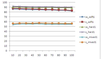
Figure-1 shows the comparison in supervised and semi-supervised learning for different k values varying from 1 to 10 for all the three vectors, namely soft, hard and mixed. In figure 1 SS_Soft1 refers to the semi-supervised learning approach for soft cluster formation. Similarly SS_hard1 and SS_mixed1 refer to the semi-supervised learning approach for hard cluster and mixed clusters respectively. S_soft1 refers to the supervised approach soft cluster, S_hard1 and S_mixed1 refers to the supervised hard and mixed cluster approach in the learning mechanism. In figure-2 the accuracy of the classifier for different values of k varying from 10 through 100 is provided. In addition to the Euclidean distance similarity measure we have other similarity measures too. But the results obtained from other similarity metrics coincides with each other. Euclidean similarity measure alone is explored in the present paper [8] [10] [15].
In order to provide enhancements to the traditional KNN algorithm the concept of variance is used. In traditional KNN algorithm all the features are given same weights in all classes, but in general not all features can be important in all classes. So taking into consideration the importance of the features in a particular class, weights are to be assigned. In this process variance of the feature term ti in class Cj is determined using the equation
12
2
(
)
|
|
ki ji
k j
ji d c
j
V
d
E
C
∈ =
−
∑
(12)
where ‘i’ takes value 1 through 14,822 and Eji is the
value of the feature item ‘i’ in the center vector of class ‘j’ and is obtained by the equation 13 which is given below
|
|
N ki k j ji
j
d d c
E
C
∈ =∑
(13)
where ‘i’ takes value 1 through 14,822
We need to find the feature distribution in all classes which can be given by the equation
2 | |
1 1
(
)
| |
c ji i j
i
E E
V
c
=−
=
∑
(14)The final weights factors to be assigned to the features can be obtained using the equation
2
(10 )
*10
i ji
ji h
h v
w =
v
(15)In the above equation wji refers to the weight vector
element of the feature item ti in the class Cj, h is an
arbitrary constant, the value used in the experiment is 5 which is in accordance to the value of the weight factors vi and vji. We find that if the value of
vji is smaller and vi is larger, then the final weight
value wji is larger.
The above steps are repeated in the process of building the semi-supervised classifier by taking only part of the training data. This is because semi-supervised learning can be applied where we have limited amount of training data or obtaining the same is very costly.
4. IMPLEMENTATION
heuristic function is employed in choosing the documents. The heurist employed was to take the document which has largest number of unique words.
In the process of building the semi-supervised classifier only 140 documents were considered, though the corpus had 8 different classes. The reason for choosing only 140 documents is because the class 4 named ‘grain’ had only 41 documents in training and 10 documents in test, so documents belonging to class ‘grain’ are removed from the corpus. Removal of the document from the corpus was done keeping in view that the classifier accuracy should not be affected due to the small number of documents in a class.
[1] gives the details of the lexicon construction phase. Lexicon set is a set of words that occurred in the training data documents. Even in case of semi-supervised learning all 5485 documents were used in the process of building the lexicon. The cardinality of the lexicon set obtained was 14,822. The objects in the lexicon set are the root words that occurred in the training data documents. We assumed the corpus is noise free, but a walk-through of the lexicon set obtained made it clear that the training data was not noise free. But no effort was put to remove the noise in the corpus. A Word pattern for each of the member of the lexicon set is obtained. The impact of the words occurrence with respect to different class labels is obtained from the word patterns. As the corpus had 7 different classes after removal of the class label ‘grain’ so each word pattern had 7 different values. For all 14,822 words in the lexicon, word patterns are obtained resulting in a vector of dimension 14,822 rows each with 7 columns.
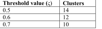
[image:6.612.314.484.105.154.2]Using the word patterns, fuzzy clusters are built. In the process of building the clusters the numbers of clusters build are decided by the threshold value ς which is provided to the algorithm as input. The threshold value attempts to find the similarity of the new word arrived with respect to the existing words, in the clusters obtained so far. Based on the similarity values obtained using the equation 9 the newly arrived word is either given a membership in one among the existing cluster or a new cluster is created. By varying the threshold value the number of clusters obtained can be controlled, for more clusters the threshold value has to be smaller, and for smaller number of clusters the threshold value has to be larger. Three different values of the threshold were explored as given in table 1 along with the correspondingly the clusters obtained are given below.
Table 1. Threshold values and clusters obtained
Threshold value (ς) Clusters
0.5 14
0.6 12
0.7 10
Once the number of clusters is formed, we implement the K-Nearest Neighbour algorithm for the text categorization.
K-Nearest Neighbour algorithm is also called as instance based learning algorithm [27]. Nearest Neighbour classifier is based on learning by analogy. In other words it is by compares a given test tuple with training tuples that are similar to it [10] [22] [23]. The training tuples are described by ‘n’ attributes. In our case the attributes are the elements in the lexicon set which are words occurred in the training document. The value of ‘n’ in out case is 14,822. Each tuple represents a point in n-dimension pattern space. When an unseen tuple is given, k-nearest neighbor classifier searches the pattern space for different values of k, which can take any value 1 through some arbitrary number. The training tuples that are closest to the unseen tuple are identified. Based on the class label of the closest tuple the value of the class label is decided. Depending on the value of k, k training tuples are used which are near to the unseen tuple. For different k tuples, the majority class label is taken, and the unseen tuple class label is declared to be the same as the majority class labels. In case of a tie, arbitrary the tie is resolved. In other words, the distance between the training and a particular test documents is measured, the class with the nearest training data is taken as the class of the test data, as here K value in K-NN is 1 as in [39]. In case of k value 2 we take two smallest distances, and if both belong to same class than the test tuple also belong to the same class as it is the nearest distance of the training data class, in case of tie an arbitrary consensus is used to resolve the conflict. Based on the similarity between the training and test tuples we obtain confusion matrix which is a good tool for analyzing, how well the classifier can classify the tuples of different classes. A confusion matrix is a plot used to evaluate the performance of a classifier in supervised learning. It is a matrix plot of the predicted versus the actual classes [25].
confusion matrix would have non-zero values and rest of the elements, very close to zero [26].
In the process of obtaining the classifier all documents belonging to the training data are processed first in case of supervised learning phase. But in case of semi-supervised learning too, the lexicon obtained from supervised learning is considered, as with alone 140 documents lexicon set cardinality would not be sufficient to handle the situation. Stemming of the words in the training data is done, and the resultant words with respect to word patterns are grouped to form clusters, thus mapping the textual data into numerical values. As the number of clusters obtained for different values of the threshold is different so the experiment was repeated 3 times in case of both semi-supervised and supervised learning, thus we obtained different clusters.
Three different types of clusters are taken into consideration, a word can be member of only single cluster, we refer to such a clusters as hard cluster, using the given below equation we obtain the membership of the hard clusters.
1 max
1
ij
t k
ζ α
=
<= <=
i
(16 )
if j= arg ( (x ))
0 otherwise
In case of soft-weighting approach we allow the word pattern to belong to more than a single cluster so rather than considering the maximum value of the function (μGα(xi)) we take
its direct value for all the clusters. In case of the soft, hard mixed-weighting (hybrid) cluster we employ the below equation where γ is the constant which dictates domination factor of the hybridization.
tij = ( ) * (1 ) *
ijH ijS
t t
γ + −γ (17)
where tijH is hard-weighting clustering approach and
tijS is the soft-weighting clustering membership
function. The value of γ can be between 0 and 1. If it is very near to 0 then the mixed weighting clustering approach coincides with the soft-clustering approach and if its value is 1 then the hard clustering approach and mixed weighting cluster results coincides with each other. Taking γ value as 0.1 the experimental results are given in figures, which are provided at the end of the paper. In case of semi-supervised learning we have only 140 documents as training data so we obtain 140 rows and the number of elements in each vector equals to the number of clusters under consideration. Since the experiment was repeated for 3 different values of the cluster we have 3
different set of clusters. Using these 140 documents series of classifiers are built iteratively. In the first iteration only 140 documents in training data are used to build the classifier. Once the classifier is built, randomly 20 documents were chosen, which were subjected to the classifier. The classifier gives the class label of the 20 documents. Now we consider that 140 documents of the initial training data and 20 documents which were subjected to the classifier are also considered as training data. Now with 160 documents as training data a new classifier is build which is expected to be superior to the first classifier built. The reason for the classifier superiority is due to the fact that the first classifier was built using 140 training documents, and the second classifier with 160 training documents. It is evident that a classifier built with more training data would give better accuracy. These steps are iteratively repeatedly for all the remaining 5305 documents, resulting in a final classifier [28]. The final classifier is subjected to the test data.
The procedure of obtaining the clusters, vector formation for test data is repeated as that of training, so all the test documents are too converted into vectors. We have 2179 vectors with the same number of elements in the vector as equal to the number of clusters as part of the test data. Once we obtain the vectors of the training and test data we apply the KNN algorithm for the vectors. We use the Euclidean measure and obtain the similarity between the training data and the test data. For different values of K we obtain the confusion matrix, in table 2 we give the accuracy for K=1 for Euclidean similarity measure for semi-supervised classifier. In table 3 the accuracy for K=1 for Euclidean similarity measure for supervised classifier is given.
In case of supervised learning too we removed the class3 which had very only 41 documents in training data. So in the training data we were left with 5444 documents. So we build a classifier with the training data which would later be subjected to the test data which has 2179 documents. The results obtained from supervised and semi-supervised classifiers were compared in the figures 1 through 6. Different similarity measures could be applied between two points or tuples say X1 and X2 which have ‘n’ component elements, which gives the similarity (closeness) between the tuples.
2 1 2 1 2 1 2 1
( , ) ( )*( ) ( )*( ) ....
Dist X Y = x x− x x− + −y y y− +y (18) In addition to the Euclidean similarity measure, other similarity measures can also be employed. Few other similarity measures that can be employed are given below.
Squared Euclidean Distance is similar to the Euclidean distance, but does not have the square-root over the summation. Mathematically square Euclidean distance is expressed as
2 1 2 1 2 1 2 1
( , ) ( )*( ) ( )*( ) ...
Dist X Y= −x x x x− + −y y y y− + (19)
Manhattan Distance is a simple similarity measure when compared to the Euclidean and square-Euclidean distance measure; it takes the summation of the absolute difference among the individual elements of the vector. Mathematical expression of Manhattan distance is expressed as
[image:8.612.314.527.91.238.2] [image:8.612.314.523.447.570.2]2 1 2 1
( , ) | | | | ... (20)
Dist X Y = x −x + y −y + Chessboard distance is also called as Chebyshev distance, Tchebychev distance), Maximum metric, it is a metric defined on a vector space where the distance between two vectors the greatest of their differences along any coordinate dimension is. It is named after Pafnuty. Mathematically the same can be expressed as
1 1 2 2
( , ) (| |, | |, ...) (21)
Dist X Y =Max x −y x −y Bray Curtis Distance is also called as Sorenson. It is defined as the fraction of absolute difference in the individual elements of the vector to the sum of the individual elements of the two vectors. The same can be expressed mathematically as
1 1 2 2
1 1 2 2
(| | | |, ...)
( , )
(| | | |, ....) (22)
x y x y Dist X Y
x y x y
− + −
=
+ + +
Canberra Distance is defined as the ratio of the sum of the absolute difference in the individual elements to the sum of the absolute values of the individual elements in the two vectors. This is mathematically expressed as
| |
( , )
| | | |
1
(23)
ik jk ik k n x x Dist X Y
x x j k
− = ∑
+ =
But in the present paper Euclidean similarity measure alone is explored. Results from [8] [10] [13] [15] showed almost similar results for different similarity measures so alone Euclidean measure is explored.
Figure 1. Supervised And Semi-Supervised Classifier Accuracy For K Values Varying From 1 To 10 For 14
Cluster
In figure 1 we draw a graph showing the accuracy of both the classifier, on X-axis we take different value of K varying from 1 through 10, in K-NN algorithm, and on Y-axis we take the accuracy of the classifier, for the 3 types of clusters soft, hard and mixed results for ς = 0.5 are shown. Similarly in figure 2 classifier accuracy for k values varying from 10 to 100 are provided for ς =0.5, that obtained 14 cluster. We find that supervised classifier outperform marginally when compared with semi-supervised classifier, giving a conclusion that in cases where limited training data alone is available semi-supervised learning paradigm can be employed to give reasonable classifier accuracy.
Figure 2. Supervised And Semi-Supervised Classifier Accuracy For K Values Varying From 10 To 100 For 14
Cluster
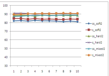
Figure 3 Supervised And Semi-Supervised Classifier Accuracy For K Values Varying From 1 To 10 For 12
Cluster
In all the figures we find marginal out-performance of supervised classifier over semi-supervised classifier. Table2 gives the accuracy of the classifier for different values of the threshold, for k value varying from 1 through 10 in case of semi-supervised classifier.
5. CONCLUSIONS
Presently bulk data is available which needs to be analyzed. In other words utilizing the existing data in decisions making makes decisions effective. The legacy data can be in textual form. In the present paper two different types of textual classifier were built, the supervised and semi-supervised learning paradigm. A blend of supervised and unsupervised classification technique was used to incorporate the fuzziness in the process of building the classifiers. Later the supervised classifier and semi-supervised classifier were compared. In the process of classifier comparison 3 types of clusters were obtained, namely soft-cluster, hard-cluster and mixed-cluster based on the word patterns. Soft-cluster is a Soft-cluster where a word can belong to more than single cluster at a given instance of time. In case of hard cluster a word can belong to a single cluster only. Mixed cluster is a hybrid of soft and hard cluster.
The results obtained from the comparison made it clear that supervised learning classifier marginally gave better accuracy compared with semi-supervised classifier, giving a bottom line that semi-supervised classifier can be applied in cases where limited amount of training data is available.
In future an attempt to decrease the size of the lexicon and see how best the classifier can learn from the training data to classify the textual data can be explored.
REFRENCES:
[1] M.A.Wajeed, T.Adilakshmi “Text Classification Using Machine Learning” Journal of Theoretical and Applied Information Technology Vol. 7 No. 2 Pages 119-123, 2009.
[2] J. Yen and R. Langari, Fuzzy Logic-Intelligence, Control, and Information. Prentice-Hall, 1999.
[3] J.S. Wang and C.S.G. Lee, “Self-Adaptive Neurofuzzy Inference Systems for Classification Applications,” IEEE Trans. Fuzzy Systems, vol. 10, no. 6, pp. 790-802, Dec. 2002.
[4] M.A.Wajeed, T.Adilakshmi “Using KNN Algorithm” Presented in International Conference on Computational Intelligence and Information Technology in november 7 – 8, 2011 and published in Springer CCIS.
[5] Correa, R.F, Ludermir, T.B. Automatic Text Categorization: Case Study, Proceedings of the VII Brazilian Symposium on Neural Networks; 2002 November; Pernambuc, Brazil.
[6] http://www.daviddlewis.com
/resources/testcollections /reuters21578.
[7] Jung-Yi Jiang, Ren-Jia Liou, Shie-Jue Lee Fuzzy Self-Constructing Feature Clustering Algorithm for Text Classification IEEE Transaction on Knowledge & Data Engineering, Vol. 23, No. 3, March 2011.
[8] M.A.Wajeed, T.Adilakshmi “Different Similarity Measures for Text Classification Using KNN” in proceedings “International Conference on Computer Communication Technology” at National Institute of Technology, Allahabad september 15-17, 2011.
[9] Fabrizio Sebastiani. Text classification, automatic. In Keith Brown (ed.), The Encyclopedia of Language and Linguistics, 2nd Edition, Vol. 14, Elsevier Science, Amsterdam, NL, 2004.
[10] M.A.Wajeed, T.Adilakshmi “Semi-Supervised Text Classification Using Enhanced KNN Algorithm” Presented in IEEE International Conference World
Congress on Information and
[11] tartarus.org/~martin/PorterStemmer.
[12] Ana Margarida de Jesus Cardoso Cachopo, “Improving Methods for Single-label Text Categorization” Phd Thesis 2007.
[13] M.A.Wajeed, T.Adilakshmi “Different Similarity Measure in Semi-Supervised text Classification” to be presented in IEEE International Conference INDICON held at Bits Pilani Hyderabad in December 16 – 18 2011 and published in IEEE Explore.
[14] Ching-man Au Yeung, Nicholas Gibbins, Nigel Shadbolt, "A k-Nearest-Neighbour Method for Classifying Web Search Results with Data in Folksonomies," wi-iat, vol. 1, pp.70-76, 2008 IEEE/WIC/ACM International Conference on Web Intelligence and Intelligent Agent Technology, 2008.
[15] M.A.Wajeed, T.Adilakshmi “Incorporating Fuzzy Clusters in Semi-Supervised Text Categorization Using Enhanced KNN Algorithm” presented in International Conference SocPros to be held at IIT Roorkee in December 20 – 22 2011 and published in Sprniger LNCS.
[16] Sumeet Agarwal, Shantanu Godbole and Diwakar Punjani “ How Much Noise is too Much: A Study in Automatic Text Classification “ in the proceedings of Seventh IEEE International Conference on Data Mining 2007.
[17] M.C. Dalmau & O.W.M. Florez. Experimental Results of the Signal Processing Approach to Distributional Clustering of Terms on Reuters-21578 Collection. 29th European Conference on IR Research, pages 678-681, 2007.
[18] Clustering of Terms on Reuters-21578 Collection,” Proc. 29th European Conf. IR Research, pp. 678-681, 2007.
[19] HIROYA TAKAMURA, “Clustering
Approaches to Text Categorization” Phd thesis 2003.
[20] W. Shang et al. t “ Novel feature selection algorithm for text categorization” / Expert Systems with Applications 33 (2007) 1–5.
[21] George Forman , “Feature Selection for Text Classification” Published as a book chapter in Computational Methods of Feature Selection 2007 CRC Press/Taylor and Francis Group.
[22] OSCAR TÄCKSTRÖM, “ An Evaluation of Bag-of-Concepts Representations in Automatic Text Classification” phd thesis 2005.
[23] D.W.Aha, D.Kibler, and M.K.Albert Instance based learning algorithms, Machine Learning, 6;37-66,1991.
[24] Padraig Cunnigham and Sarah Jane Delany “K-Nearest Neighbour Classifiers” Technical Report UCD-CSI 2007-4.
[25] Data Normalization
http://abbottanalytics.blogspot.com/2009/0 4-why-normalization-matters-with-k-means.html.
[26] Cai, L.and Hofmann,T. Hierarchical Document Categorization with Support Vector Machines.In Proceedings of the ACM Conference on Information and Knowledge Management, pages 78-87, 2004.
[27] Lihua Song, Jidong Zhang, An Improved K-Nearest Neighbor System and Its Application to Text Classification [J]. Applied Science and Technology, 2002,March,171-174.
[28] A.Azran.The rendezvous
algorithm:Multiclass semi-supervised learning with markov random walks.In Proceedings of the 24th International Conference on Machine Learning, 2007.
[29] J. Yen and R. Langari, Fuzzy Logic-Intelligence, Control, and Information. Prentice-Hall, 1999.
[30] J.S. Wang and C.S.G. Lee, “Self-Adaptive Neuro fuzzy Inference Systems for Classification Applications,” IEEE Trans. Fuzzy Systems, vol. 10, no. 6, pp. 790-802, Dec. 2002.
[31] M.A.Wajeed, T.Adilakshmi “Supervised and Semi-supervised Learning in Text Classification Using Enhanced KNN Algorithm (A Comparative study of
Supervised and Semi-supervised
Classification in Text Categorization) “ in International Journal of Intelligent Systems Technologies and Applications journal, published by inderscience
[32] Ya Xue,Xuejun Liao and Lawrence Carin, “ Multi-Task Learning for Classification with Dirichlet Process Priors” , Journal of Machine Learning Research 8 (2007) 35-63.
[33] Martin Sewell, “ Feature Selection”, 2007.
for Classification and Indexing” , in Proceedings of Conference on Information & Knowledge Management, Napa, CA Oct 27, 2008.
[35] Abdelwadood Moh'd A MESLEH ,”Chi Square Feature Extraction Based Svms Arabic Language Text Categorization System”, Journal of Computer Science 3 (6): 430-435, 2007.
[36] Olivier Chapelle, Bernhard Scholkopf, Alexander Zien, “Semi-Supervised Learning”, The MIT Press Cambridge, Massachusetts London, 2006.
[37] Lifei Chen, Yanfang Ye, Qingshan Jiang, “A New Centroid-Based Classifier for Text Categorization” in proceeding of 22nd International Conference on Advanced Information Networking and Applications – Workshops 2008.
[38] P Cunningham et al “K-Nearest Neighbour Classifier”, Technical Report, 2007.
[39] Raschka “ Naive Bayes and Text Classification I-Introduction and Theory”, Article, 04 October 2014.
[40] Wang et al. "Text classification with heterogeneous information network kernels." Thirtieth AAAI Conference on Artificial Intelligence. 2016.
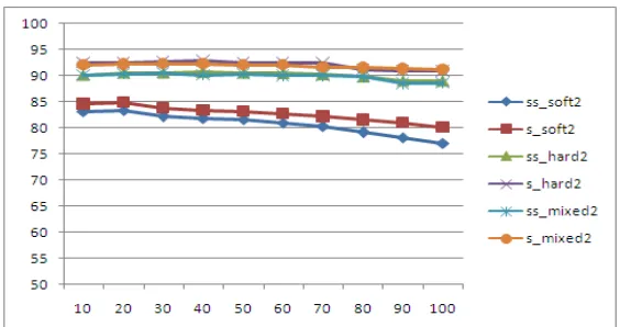
Figure 4 Supervised and Semi-supervised Classifier accuracy for K values varying from 10 to 100 for 12 cluster
[image:12.612.157.457.437.575.2]Figure 5 Supervised and Semi-supervised Classifier accuracy for K values varying from 1 to 10 for 10 cluster
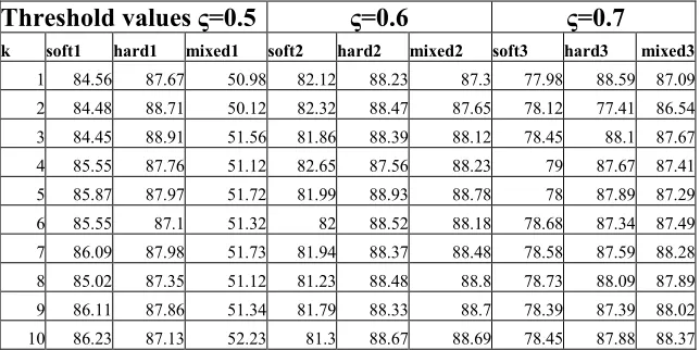
Table 2. Accuracy of semi-supervised classifier for different cluster types for different threshold vlue for K value varying from 1 to 10
Table 3. Accuracy of the supervised classifier for different cluster types for different threshold value for K value varying from 1 to 10.
Threshold values ς=0.5
ς=0.6
ς=0.7
k soft1 hard1 mixed1 soft2 hard2 mixed2 soft3 hard3 mixed3
1 84.56 87.67 50.98 82.12 88.23 87.3 77.98 88.59 87.09
2 84.48 88.71 50.12 82.32 88.47 87.65 78.12 77.41 86.54
3 84.45 88.91 51.56 81.86 88.39 88.12 78.45 88.1 87.67
4 85.55 87.76 51.12 82.65 87.56 88.23 79 87.67 87.41
5 85.87 87.97 51.72 81.99 88.93 88.78 78 87.89 87.29
6 85.55 87.1 51.32 82 88.52 88.18 78.68 87.34 87.49
7 86.09 87.98 51.73 81.94 88.37 88.48 78.58 87.59 88.28
8 85.02 87.35 51.12 81.23 88.48 88.8 78.73 88.09 87.89
9 86.11 87.86 51.34 81.79 88.33 88.7 78.39 87.39 88.02
10 86.23 87.13 52.23 81.3 88.67 88.69 78.45 87.88 88.37
Threshold values ς=0.5
ς=0.6
ς=0.7
k soft1 hard1 mixed1 soft2 hard2 mixed2 soft3 hard3 mixed3
1 86.28 89.26 53.37 88.87 90.87 89.68 82.28 91.09 89.72
2 86.25 90.48 53.21 84.73 90.96 89.88 81.27 90.41 89.49
3 86.24 90.69 54.42 83.83 90.63 91.34 81.41 91.05 90.41
4 86.89 90.12 54.23 84.98 89.82 91.21 82 91.87 90.54
5 87.12 90.23 54.67 83.88 90.62 91.67 81.96 91.69 90.18
6 87.05 89.27 54.34 84.21 90.77 91.4 81.68 92.01 90.54
7 88.04 89.46 54.59 84.04 90.56 91.54 81.54 91.78 90.41
8 87.89 89.22 54.31 83.78 90.49 91.97 81.73 92.19 90.73
9 88.21 89.62 54.49 84.22 90.83 91.88 81.82 91.64 90.22
[image:13.612.146.468.347.508.2]