Munich Personal RePEc Archive
Regional inflation and industrial
structure in monetary union
Nagayasu, Jun
1 March 2012
Online at
https://mpra.ub.uni-muenchen.de/37310/
Title: Regional Inflation and Industrial Structure in Monetary Union
Date: March 2012
Abstract:
It is often argued that an optimal currency area requires homogeneous regional inflation. However, previous empirical studies point out heterogeneity in sectoral inflation and geographical concentration of industries within a monetary union. It follows that there must be a difference in regional inflation in such a union. We examine this view using regional data from Japan which has experienced a period of rapid change in industrial structure, and show that economic structure is closely related to heterogeneous regional inflation. This study suggests that heterogeneous inflation can be a prevailing and long-lasting phenomenon in a monetary union.
Keywords: Regional inflation, Monetary union, Optimal currency area, Industrial
structure
1. Introduction
This paper empirically analyzes the behavior of time-varying correlations of regional
inflation in a monetary union; in particular we focus on its relationship with industrial
structure. Mundell (1961) argued that an optimal currency area requires homogeneous
regional inflation in order to avoid asymmetric effects of a single monetary policy and
exogenous shocks to the regions. Furthermore, homogeneous inflation is expected to
prevail in a monetary union, due to the increased economic integration after forming the
single currency area. The presence of homogeneity in regional inflation in a monetary
union is thus widely accepted by researchers and policymakers and is included in the
Maastricht Treaty as a prerequisite for joining the euro area.
However, there is increasing evidence of heterogeneous regional inflation
within a monetary union using the comprehensive coverage of price data like the
Consumer Price Index (CPI).1 Kocenda and Papell (1997), Homes (2002), and Busetti
et al (2006) reported evidence of inflation convergence in the pre-euro period. However,
this trend has changed since the introduction of the euro, and regional inflation is
diverging, forming two convergence clubs in the European Monetary Union, EMU
(Busetti et al 2006).2 Similarly, Nagayasu (2011) presented evidence of heterogeneous
inflation and non-convergence of prices using Japanese regional data.
There are some economic explanations for heterogeneous regional inflation.
Recent studies (e.g., Aoki 2001; Fuchi and Watanabe 2001; Altissimo et al 2007; Leith
1 There is more evidence in favor of inflation (price) convergence from studies utilizing
product-specific data. For example, Golberg and Verboven (2005) show that both levels of and changes in car prices are converging in Europe.
2 Inflation divergence and price convergence can take place simultaneously in the process of
monetary integration since a low-price region may experience higher inflation to catch up with a high-price region. In this connection, Faber and Stokman (2009) showed a declining trend in price dispersion among members of the EMU, but there is no evidence that this price adjustment
and Malley 2007; Imbs et al 2011) have underlined different levels of inflation
persistence and of inflation itself across industries. Among economic sectors, the service
sector tends to exhibit higher inflation persistence. When sectoral inflation persistence
and thus sectoral inflation rates are different, there must be differences in regional
inflation because there is evidence of dissimilarity in the industrial structure in the
European Union (EU) (Brulhart 2001). Thus these studies imply that in the absence of
convergence in industrial structure, regional inflation rates do not converge even after
the establishment of monetary union.
Against this background, we focus on two main issues. First, we analyze if
there is any difference in industrial structure using regional data from Japan. In the
nearly 70 years since the end of the war, the industrial structure has changed
dramatically. Nowadays the tertiary (rather than the secondary) sector is dominant in the
country, while the primary industries have been stagnating and play an insignificant role
in total economic activities. Second, if there are indeed significant differences in
industrial structure among regions, then we examine whether it can explain the
correlations of regional inflation. Thus this study will fill a gap between research in the
areas of international trade, monetary economics and international finance.
This study is also rather distinctive because of our area choice. The Japanese
regions are believed to be relatively homogenous in terms of culture (e.g., language,
religion, race, and political and legal systems) by international standards. Furthermore,
there are no trade barriers such as tariffs on tradable goods nor legal barriers to free
movement of labor between regions. Findings from regions that are likely to meet the
conditions of an optimal currency area will have significant policy implications for
2. Regional inflation
We study regional inflation from 1976Q4 to 2008Q4 measuring annual changes (△pt =
ln(pt / pt-4)) in the Consumer Price Index (CPI (p)). This sample period begins when data
from Okinawa, which was returned to Japan in 1972, became available, and the
end-of-period is determined by the data availability of our explanatory variables which
will be discussed later. Our dataset consists of 10 regions; Hokkaido, Tohoku, Kanto,
Hokuriku, Tokai, Kinki, Chugoku, Shikoku, Kyushu and Okinawa, following the
classification methodology used by the Ministry of Internal Affairs and
Communications which is responsible for compilation of the CPI. The appendix
describes the data and summarizes the definition of the regions in which all 47
prefectures are included.
Figure 1 shows a very similar movement of regional inflation with occasional
deflationary episodes; a relatively high level of inflation in the 1970s and early 1980s in
response to the oil crises, and low inflation in more recent periods reflecting weak
economic recovery after the bursting of the bubble in the financial and real estate
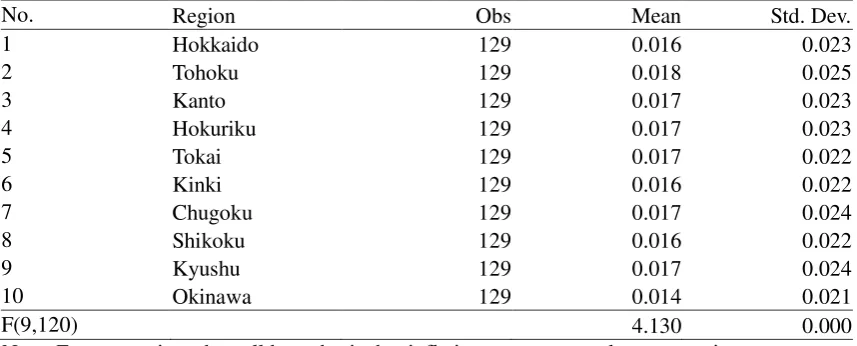
markets. While inflation rates and their volatility look very similar across regions (Table
1), Okinawa, which lags behind other regions in terms of economic development, has
experienced the lowest inflation. Furthermore, F tests in this table suggest that regional
inflation is indeed different, a result consistent with Nagayasu (2011). While the
difference in regional inflation is at most 0.4% (Table 1) and seems insignificant
compared with one in Europe,3 we confirm statistically significant heterogeneity in
regional inflation even in this country with a relatively small landmass and similar
3 During 1999-2010, the difference between the maximum and minimum inflation rates was 4.1% in
culture—a result consistent from other countries/monetary unions (e.g., Busetti et al
2006).
While we shall go into details later on, our result is also in line with
heterogeneous economic structure among regions. Heterogeneous sectoral inflation in a
monetary union is observed worldwide; for example, Fuchi and Watanabe (2001) and
Altissimo et al (2007) showed from Japanese and European data respectively that there
is a significant difference in sectoral inflation within a region/country, and services tend
to exhibit higher inflation persistence than industrial goods. In the presence of industry
concentration in a certain region, there likely exists heterogeneous inflation.
Furthermore, in order to show interaction between regional inflation, its
variance is decomposed using the method suggested by Diebold and Yilmaz (2009). For
presentation purposes, Table 2 summarizes the results according to the size of regional
economies measured by the GDP and reports evidence of inflation spillovers. This
variance decomposition is carried out using the residuals from the 4th order 10 variable
Vector Auto-Regressor (VAR): xt = φ1xt-1 +φ2xt-2+φ3xt-3+φ4xt-4+ εt or xt = A(L)ut in the
moving average form, where L is a lag operator. The Cholesky decomposition method is
employed to calculate the contribution of region i’s inflation variance to the
4-step-ahead forecasting residual variance of region j (i≠j, i=1,…,10 and j=1,…,10). In
short, spillover effects are calculated as:
4 10 2 , 0 , 1 4
0
100
( ' ) h ij h i j
h h h
a Spillover
trace A A
(1)where ah,ij is an element of A:
,11 ,12 ,110
,21 ,210
,101 ,102 ,1010
h h h
h h
h h h
a a a
a a
A
a a a
forecast. Thus equation (1) is a ratio of the total spillover to the variation of the total
forecast error.
Table 2 shows that regional inflation in Kanto which includes Tokyo (the
nation’s capital) is least affected by other regions, and is mostly generated by Kanto
itself. While other regional inflation is also generally most affected by itself, influence
from other regions is substantial. Interestingly, like Kanto, Okinawa is also less affected
by inflation in other regions.4 In short, countrywide inflation is dominated by the
inflation in Kanto.5
Finally, the moving-window correlations of regional inflation are calculated
with a different window size (5, 10 and 20) in order to check the sensitivity of our final
results to the window size. Figure 2 plots correlations from a window size of 10 and
shows that it is time-varying and has a high value (often more than 0.5). But
correlations tended to be low when there were large economic shocks such as banking
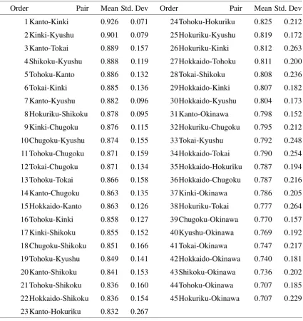
problems with high non-performing loans (2000) and Lehman Shock (2008). Table 3
presents the average of correlations for each pair of regions. The highest correlation can
be obtained between Kanto and Kinki—industrial regions with the present and former
capital cities. The lowest level is found between Hokuriku and Okinawa, and
interestingly all pairings with Okinawa are listed in the low correlation group. This
again characterizes the unique position of Okinawa. In order to better understand the
characteristics of regions, we shall look into their industrial structure next.
3. Diversification of Industrial structure
Production concentration is important in our study since recent studies of inflation in the
4
In general, the result remains unchanged even if the order of variables in the specification has altered.
5
New Keynesian framework emphasized differences in the persistence of sectoral
inflation. When inflation persistence and thus inflation rates are different among
industrial sectors and if regions specify production of goods and services, monetary
union likely faces long-lasting heterogeneous regional inflation.
There are several economic theories which would lead one to expect a country
(region) to specialize in the production of particular goods and services. For example,
David Ricardo proposed the concept of comparative advantage in order to explain
international trade, and predicted that a country specializes in the production of products
according to technological differences. In contrast, Heckscher-Ohlin model pointed to
differences in factor endowments in countries as an engine of international trade. A
country will specialize in the production of products that utilize economic factors that
are internationally more affluent.
Marshall (1920) and Krugman (1991) provided three further theoretical
explanations of high localization of industries. First, the proximity of firms in the same
industry creates a labor market pool. Since these firms seek similar types of skilled
workers, the labor market pool helps reduce the possibilities of mismatching and
functions to introduce flexibility into the labor market. Second, the agglomeration of
similar firms creates a more efficient market since firms can have easier access to
specialized intermediate inputs and services. Third, firms can benefit more from
knowledge spillover by locating close to each other. In this regard, Yamawaki (2002)
reported that Japanese small firms consider, among other things, the location of leading
firms nearby and the availability of relevant skilled workers as key factors in their
decision-making about location.
value-added shares6 and the classification method of the Cabinet Office, Government
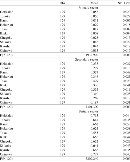
of Japan (i.e., the primary, secondary and tertiary sectors). Table 4 shows the proportion
of all three sectors across the regions. The primary sector is relatively more important in
the northern regions (Hokkaido and Tohoku) which are known to produce agricultural
products, but the secondary sector plays a more significant role throughout Japan, in
particular Tokai where the headquarters of Toyota are located. However, it is the tertiary
sector which has the highest ratio to GDP, particularly in Okinawa. Thus although Japan
may often be regarded as a manufacturing country with many internationally
competitive firms, it is the service sector which contributes most to overall economic
activity.
Furthermore, the proportion of the tertiary sector has been increasing over time,
matched by a decline in that of the primary and secondary sectors (Figure 3). (This
figure shows the trend of each sector at the national level.) More specifically, while
some industries such as the semiconductor as well as the processing and assembly
industries (e.g., cars, semiconductors, general electrical machines) expanded rapidly
until the 1980s, the secondary sector has shown a steady decline during our period, and
the decline accelerated in the 1990s during the economic slowdown. Despite a slow
adjustment due to the rigidity in the labor market however, there have been notable
advances in the information and technology industry, an area which is closely related to
the tertiary sector. Therefore, it is expected that in the future the tertiary sector will
maintain its significant presence in the Japanese economy.
We study if there is divergence in production specialization in Japanese regions
6
using the β convergence criterion often used in economic growth literature.7
This
criterion suggests that convergence in industrial structure takes place, for example,
when a region with a low contribution from the primary sector experiences higher
growth in the ratio of the primary sector’s activities-to-GDP than a region with a high
contribution from this sector. The concept of β convergence can be summarized as:
1 1
(yit /yit ) (yit )uit (2)
where yit represents the ratio of real sectoral GDP to total GDP for region i at time t and
the residual u has zero mean with a constant variance. Parameter α captures a
steady-state value and thus here is cross-sectionally constant (i.e., absolute
convergence). The condition of convergence requires 0 < β < 1 which indicates a
negative correlation between changes in y and lagged y. A more general form can be
written as:
4
1 1 1
1
( it / it ) ( it ) j( it j/ it j ) it j
y y y y y u
(3)where δ = - β and the lagged endogenous variable is included in order to deal with
autocorrelation. The convergence condition thus becomes -1 < δ < 0. Since our data are
from the same country and are thus expected to be highly correlated with one another,
we shall estimate equation (3) by the Seemingly Unrelated Regression (SUR) method in
order to capture the cross-sectional correlation in the residual terms a la Breuer et al
(2001). For presentation purposes, we also present results from replacing α with αi
(conditional convergence) in equations (3) with and without the lagged endogenous
variable.
7
Table 5 presents parameter δ and fixed terms α and αi estimated for each sector
along with the standard errors based on the bootstrap method since statistics do not
follow a conventional distribution. In general, we can observe convergence in the
primary sector regardless of the specification of the steady-state, and divergence in the
secondary and tertiary sectors. This observation is supported by the signs and statistical
significance of our estimates. Parameter δ is positive for the tertiary sector which
implies β < 0. While δ is negative for the secondary sector, this parameter is statistically
insignificant. These findings support non-convergence of industry structure for these
sectors. In contrast, δ is negative and significant for the primary sector, raising evidence
of convergence in its sector. This is consistent with the fact that activities in the primary
sector like agriculture, which contributes least to overall economic activity, has been
decreasing throughout Japan. In contrast, the manufacturing and service sectors seem to
be concentrated in certain (often rural) areas. This conclusion remained unchanged even
when the different size of lag orders (j=1 to 4 in equation (2)) is used.8
The non-convergence of industry structure is observed in trade unions in
Europe too. For European countries, Brulhart (2001) for example looked at the
manufacturing industry in 13 European countries over the period of 1972-1996, and
reported that sectoral employment specialization has been increasing over time. Gugler
and Pfaffermayr (2004) showed that for 14 EU countries over the period 1985-98 while
there is evidence of convergence in productivity, industry structure remains unchanged.
Similarly, Brulhart and Traeger (2005) showed that there was no significant change in
the geographical concentration of employment and market services between 1975-2000
8 We also consider equation (3) with the a priori assumption of homogeneous α
i (i.e., α1=α2=…α10)
and heterogeneous δi. The general conclusion remains the same as those from the assumption
in the EU, but there was evidence of convergence in the manufacturing sector. In the
international context, Rodrik (2011) argued about the importance of the investigation
into economic convergence at the sectoral level; the conclusion of convergence is
sensitive however to the choice of industries.
4. Empirical relationship
Here we shall examine the relationship between the correlations of regional inflation
and economic factors including the industrial structure of the regions. More precisely,
we consider economic variables such as deposits and demographic changes which are
expected to capture the unique characteristics of each region.9
The Japanese economy and the society cannot be discussed without
considering demographic changes. Japan has experienced a rapid increase over recent
years in the aged proportion of its population. With a low birthrate (less than 2% since
1975) and longevity, there is a relatively small workforce in the country. This was
recently exacerbated by the retirement of the baby-boom generations. This phenomenon
has had serious economic and social impacts on the society, putting further pressure on
the national budget, due to increased outlay from the social security system and the
social safety net, which are already in a rather fragile state.
Demographic changes have affected living patterns, and underpopulation
(Kasoka) has become a common phenomenon throughout Japan. At the national level,
underpopulated cities (including villages and towns) have increased from 38.3% in
9 We also considered geographical proximity in this section by introducing to equation (4) a dummy
1990 to 45% in 2011.10 Furthermore, such cities are unevenly distributed across the
country and, while a majority of prefectures have experienced further underpopulation,
there are 5 out of 47 prefectures which have improved their situation during this
period.11 Increases in job opportunities as well as ‘while still expensive more affordable’
living environments motivated residents in rural areas to move to big cities. As a result,
a high dependency ratio (i.e., a high proportion of retirees and children) is often seen in
the countryside.
Finally, the size of bank deposits is considered in order to capture similarity
across regions. Generally, large economies including Kanto and Kinki regions tend to
have high bank deposits. This variable is closely related to demographic changes; recent
studies (Horioka 2010) pointed out that there is a negative relationship between bank
deposits and the proportion of dependents. In particular, retirees have started ‘dis-saving’
(spending) their deposits to cover their living expenses.
Using these data and the correlation of regional inflation (Corr(Δpijt) )
calculated with several window sizes, we estimate the following general specification
for panel data:
1 2
3 4
( ) | | | _ _ |
| |
ijt it jt it jt
it jt ijt
Corr p Ind Ind Work pop Work pop Deposit Deposit t u
(4)
where Ind is a change in a proportion of industrial structure for a particular sector (e.g.,
real GDP for the primary sector/Total GDP), Work_pop is a change in a demographic
ratio using the definition of workforce as from 15 to 65 years old (i.e.,
Workforce/Population), and Deposits is a change in demand deposits, Subscripts i and j
10
See http://www.kaso-net.or.jp/index.htm for definition and further information about
underpopulation in Japan. Among other conditions a city is considered underpopulated when more than a certain number of residents have moved away.
11
represent region (i≠j). The absolute value of these ratios is examined in order to
capture the proximity of regions: the regions are said to be similar, when this absolute
value becomes small (approaches zero). In order to take account of endogeneity issues,
equation (4) will be estimated by the Generalized Method of Moments (GMM). Davis
et al (2011), for example, showed that industrial structure is affected by inflation in
OECD countries, a direction of causality opposite to (4).
Table 6 summarizes our empirical results and also lists the instruments used in
the 2-step GMM estimation. The standard errors (SE) in this table are robust to
heterogeneity and autocorrelation. We used only the secondary and tertiary sectors in
this analysis since the primary sector is insignificant in size and is converging within a
country. Generally the results are consistent with our expectations; all key variables
have a correct sign often with statistical significance. Namely, regional differences in
industrial structure, demographic factors and deposits are negatively correlated with
regional inflation. Thus, we confirm that a similar level of regional inflation can be
observed among similar regions in terms of these three criteria. This result is generally
unchanged even when correlations with a different window size are employed.
This is also consistent with our preliminary analysis of the data. Due to its
heavy reliance on services (e.g., tourism) for geographical and historical reasons,
Okinawa had a rather distinctive profile with the lowest and highest ratios for the
secondary and tertiary sectors respectively (Table 4). This distinguishing factor seems to
contribute to the low correlation of inflation with other regions.
Since industrial structure shows no sign of convergence in general, we expect
the low correlations of regional inflation among heterogeneous regions in future too.
even among the Japanese regions which are often considered, by international standards,
to be homogenous in many respects.
The GMM results are known to be sensitive to the choice of instrumental
variables, and recent studies emphasize the importance of checking both the order (i.e.,
the number of instruments greater than the unknown parameters) and rank conditions in
order to see the appropriateness of instruments. In this connection, the
under-identification (Kleibergen and Paap 2006) and weak identification (Stock and
Yogo 2005) tests are implemented in this study.12 All these tests in additional to the
conventional Hansen J test confirm that our instruments are statistically appropriate and
thus our results are reliable.
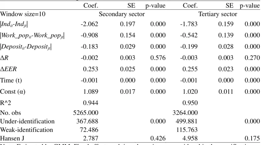
Finally, we consider extra variables which capture the financing costs of firms
since there is evidence that regional inflation responds differently to exogenous shocks
which are common to regions (Nagayasu 2011) and firms respond heterogeneously to
increases in financing costs (Berman et al 2009; Dhyne and Druant 2010). Furthermore,
studies on Pricing-to-Market give rise to evidence of partial exchange rate pass-through
into import prices in advanced countries although this pass-through effect has been
declining in recent years (Warmedinger 2004, Campa and Golderg 2005, Otani et al
2006). In this regard, we use the call rate (R) and a nominal effective exchange rate
(EER) which is expressed in terms of yen.
The results are summarized in Table 7. Again, the model is estimated by the
GMM, and instrumental variables are explained in the table. Increases in financial costs
are represented by a rise in R and a decline in EER (i.e., yen depreciation). In such
circumstances, we expect a low level of inflation correlation and thus a negative
12
(positive) relationship between inflation correlation and the call rate (the exchange rate).
Using the growth rates of these variables, our data confirm this theoretical expectation;
at times of tight monetary policies and yen depreciation, heterogeneities become more
apparent in regional inflation. In terms of statistical significance, the exchange rate is
reported to be more influential over inflation correlations. With respect to variables in
the absolute value, the results remain the same as before and indicate high inflation
correlation among similar regions.
5. Summary and Discussion
This paper empirically investigated the relationship between regional inflation and
industrial structure using Japanese regional data, and reported mainly two findings. First,
industrial structure has been changing in Japan; while the primary sector has been
diminishing throughout Japan, there is evidence of non-convergence in the secondary
and tertiary sectors which dominate the economy. Second, given this, we found that
there is a strong link between the correlations of regional inflation and changes in
industrial structure. Since there is no sign of convergence in the key sectors among
regions, the phenomenon of heterogeneous inflation is likely to prevail in years to come.
Third, our data suggest that inflation correlations tend to decline at times of increasing
financial cost, which also reflects the different economic structures in each region.
While this study focuses on Japanese regions, our findings provide potentially
useful information for countries considering joining the euro area. Since there is no
strong sign of convergence in industrial structure in Europe, our study predicts
continuously heterogeneous inflation in the future. If so, economic imbalances must be
dealt with by other means such as fiscal transfers—a lack of which likely makes a
size of intergovernmental fiscal transfers in Japan (from central to local governments) is
one of the highest among the major industrialized nations.13 Without such a transfer
mechanism, prevented in the euro area by the Lisbon Treaty, stronger discipline
regarding inflation and price convergence is necessary to maintain the single currency
area. In contrast, our findings may have limited policy implications for the Japanese
monetary authorities. This is because inflation spillover from the urban (e.g., Kanto
area) to other regions is substantial. Such circumstances may justify close monitoring of
inflation developments in Kanto, even in order to control inflation in other areas.
13
References
Altissimo, F., B. Mojon and P. Zaffaroni, 2007. Fast Micro and Slow Macro: Can
Aggregation Explain the Persistence of Inflation? European Central Bank Working
Paper No. 729.
Aoki, K. 2001. Optimal Monetary Policy Responses to Relative-price Changes. Journal
of Monetary Economics 48: 55-80.
Barro, R. J. and X. Sala-i-Martin. 1999. Economic Growth. Cambridge: MIT Press.
Berman, N., P. Martin and T. Mayer. 2009. How Do Different Exporters to React to
Exchange Rate Changes? Theory, Empirics and Aggregate Implications. Centre for
Economic Policy Research Discussion Paper No. 7493.
Breuer, J. B., R. McNown and M. S. Wallace. 2001. Misleading Inferences from Panel
Unit Root Tests with an Illustration from Purchasing Power Parity. Review of
International Economics 9: 482-493.
Brulhart, M. 2001. Growing Alike or Growing Apart? Industrial Specialization of EU
Countries, Wyplosz, C. ed. The Impact of EMU on Europe and the Developing
Countries: Oxford University Press.
Brulhart, M. and R. Traeger. 2005. An Account of Geographic Concentration Patterns in
Europe. Regional Science and Urban Economics 35: 597-624.
Busetti, F., L. Forni, A. Harvey and F. Venditti. 2006. Inflation Convergence and
Divergence within the European Monetary Union. European Central Bank Working
Paper No. 574.
Campa, J. M. and L. S. Goldberg. 2005. Exchange Rate Pass-through into Import Prices.
Review of Economics and Statistics 87: 679-690.
Cuaresma, J. C., B. Egert and M. A. Silgoner. 2007. Price Level Convergence in
Europe: Did the Introduction of the Euro Matter? Monetary Policy & the Economy Q1:
100-113.
Davis, G. K., D. Hineline and B. E. Kanago. 2011. Inflation and Real Sectoral Output
Shares: Dynamic Panel Model Evidence from Seven OECD Countries. Journal of
Macroeconomics 33: 607-619.
Dhyne, E. and M. Druant. 2010. Wages, Labor or Prices: How do Firms React Shocks?
Diebold, F. X. and K. Yilmaz. 2009. Measuring Financial Asset Returns and Volatility
Spillovers, with Application to Global Equity Markets. Economic Journal 119: 159-171.
Faber, R. P.and AD C. J. Stokman. 2009. A Short History of Price Level Convergence
in Europe. Journal of Money, Credit, and Banking 41: 461-477.
Fuchi, H. and T. Watanabe. 2001. Phillips Curve and Price Persistence: Results from
Sectoral Data (in Japanese). Institute for Monetary and Economic Studies Discussion
Paper No. 2001-J-29, Bank of Japan.
Goldberg, P. K. and F. Verboven. 2005. Market Integration and Convergence to the Law
of One Price: Evidence from the European Car Market. Journal of International
Economics 65: 49-73.
Gugler, K. and M. Pfaffermayr. 2004. Convergence in Structure and Productivity in
European Manufacturing? German Economic Review 5: 61-79.
Homes, M. J. 2002. Panel Data Evidence on Inflation Convergence in the European
Union. Applied Economics Letters 9: 155-158.
Horioka, C. Y. 2010. The (Dis)saving Behavior of the Aged in Japan. Japan and the
World Economy 22: 151-158
Imbs, J., E. Jondeau and F. Pelgrin. 2011. Sectoral Phillips Curves and the Aggregate
Phillips Curve. Journal of Monetary Economics, forthcoming.
Kleibergen, F. and R. Paap. 2006. Generalized Reduced Rank Tests Using the
Singular-value Decomposition. Journal of Econometrics 127: 97-126.
Kocenda, E. and D. Papell. 1997. Inflation Convergence within the European Union: A
Panel Data Analysis. International Journal of Finance and Economics 2: 189-98.
Krugman, P. 1991. Geography and Trade. Cambridge: MIT Press.
Leith, C. and J. Malley. 2007. A Sectoral Analysis of Price-setting Behavior in US
Manufacturing Industries. Review of Economics and Statistics 89: 335-342.
Marshall, A. 1920. Principles of Economics. London: Macmillan.
Mundell, R. 1961. A Theory of Optimal Currency Areas. American Economic Review
51: 657-665.
Nagayasu, J. 2011. Heterogeneity and Convergence of Regional Inflation (prices).
Journal of Macroeconomics 33: 711-723.
Rate Pass-through: Further Evidence from Japan’s Import Prices. Monetary Economic
Studies. 61-75.
Rodrik, D. 2011. Unconditional Convergence. Preliminary draft, Harvard University.
Stock, J. H. and M. Yogo. 2005. Testing for Weak Instruments in Linear IV Regression.
In Identification and Inference for Econometric Models: Essays in Honor of Thomas
Rothenberg. Andrews, D. W. K. and J. H. Stock eds., 80-108, Cambridge: Cambridge
University Press.
Warmedinger, T. 2004. Import Prices and Pricing-to-market Effects in the Euro Area.
European Central Bank Working Paper Series No. 299.
Yamawaki, H. 2002. The Evolution and Structure of Industrial Clusters in Japan. Small
Appendix. Data Description
Regional classification (based on the Statistics Bureau, the Ministry of Internal Affairs and
Communications)
Region Prefectures
Hokkaido Hokkaido
Tohoku Aomori, Iwate, Miyagi, Akita, Yamagata, Fukushima
Kanto Ibaraki, Tochigi, Gunma, Saitama, Chiba, Tokyo, Kanagawa,
Yamanashi, Nagano
Hokuriku Niigata, Toyama, Ishikawa, Fukui
Tokai Gifu, Shizuoka, Aichi, Mie
Kinki Shiga, Kyoto, Osaka, Hyogo, Nara, Wakayama
Chugoku Tottori, Shimane, Okayama, Hiroshima, Yamaguchi
Shikoku Tokushima, Kagawa, Ehime, Kochi
Kyushu Fukuoka, Saga, Nagasaki, Kumamoto, Oita, Miyazaki, Kagoshima
Okinawa Okinawa
Regional CPI: Monthly data are obtained from the Statistics Bureau, the Ministry of Internal
Affairs and Communications (MIAC). Quarterly data are based on the end-of-period.
Regional/Sectoral GDP: Annual data are obtained from the Cabinet Office, Government of
Japan. Two datasets are combined using year 1999 as a benchmark. Annual data are converted
to quarterly data and real data using regional CPI since sectoral price data consistent with our
regional classification are not available.
Population/Dependency ratio: Annual data are obtained from the e-Stat organized by the MIAC.
http://www.e-stat.go.jp/SG1/chiiki/ToukeiDataSelectDispatchAction.do.
Deposits: Demand deposits are from the Bank of Japan.
Interest rates: call rates from the Nikkei Needs.
Effective exchange rates: nominal effective exchange rates from the International Financial
Table 1. Basic Statistics of Regional Inflation and Industries
No. Region Obs Mean Std. Dev.
1 Hokkaido 129 0.016 0.023
2 Tohoku 129 0.018 0.025
3 Kanto 129 0.017 0.023
4 Hokuriku 129 0.017 0.023
5 Tokai 129 0.017 0.022
6 Kinki 129 0.016 0.022
7 Chugoku 129 0.017 0.024
8 Shikoku 129 0.016 0.022
9 Kyushu 129 0.017 0.024
10 Okinawa 129 0.014 0.021
F(9,120) 4.130 0.000
Tables 2. Regional Inflation
Note: The order of regions is based on the scale of GDP. Based on the fourth period ahead
forecasting model.
% From
To K an to K in k i T o k ai K y u sh u T o ho ku C h ug ok u H o ku ri k u H o kk ai d o S h ik o ku O k in aw a F ro m O th er s
Table 3. Correlation Level/levels
Order Pair Mean Std. Dev Order Pair Mean Std. Dev
1 Kanto-Kinki 0.926 0.071 24 Tohoku-Hokuriku 0.825 0.212
2 Kinki-Kyushu 0.901 0.079 25 Hokuriku-Kyushu 0.819 0.172
3 Kanto-Tokai 0.889 0.157 26 Hokuriku-Kinki 0.812 0.263
4 Shikoku-Kyushu 0.888 0.119 27 Hokkaido-Tohoku 0.811 0.200
5 Tohoku-Kanto 0.886 0.132 28 Tokai-Shikoku 0.808 0.236
6 Tokai-Kinki 0.885 0.136 29 Hokkaido-Kinki 0.807 0.182
7 Kanto-Kyushu 0.882 0.096 30 Hokkaido-Kyushu 0.804 0.173
8 Hokuriku-Shikoku 0.878 0.095 31 Kanto-Okinawa 0.798 0.152
9 Kinki-Chugoku 0.876 0.115 32 Hokuriku-Chugoku 0.795 0.212
10 Chugoku-Kyushu 0.874 0.155 33 Tokai-Kyushu 0.792 0.248
11 Tohoku-Chugoku 0.871 0.159 34 Hokkaido-Tokai 0.790 0.254
12 Tokai-Chugoku 0.871 0.134 35 Hokkaido-Hokuriku 0.787 0.194
13 Tohoku-Tokai 0.866 0.158 36 Hokkaido-Chugoku 0.787 0.216
14 Kanto-Chugoku 0.863 0.135 37 Kinki-Okinawa 0.786 0.205
15 Hokkaido-Kanto 0.863 0.126 38 Hokuriku-Tokai 0.777 0.264
16 Tohoku-Kinki 0.858 0.127 39 Chugoku-Okinawa 0.770 0.157
17 Kinki-Shikoku 0.855 0.152 40 Kyushu-Okinawa 0.769 0.192
18 Chugoku-Shikoku 0.851 0.166 41 Tokai-Okinawa 0.747 0.217
19 Tohoku-Kyushu 0.849 0.141 42 Hokkaido-Okinawa 0.740 0.181
20 Kanto-Shikoku 0.841 0.153 43 Shikoku-Okinawa 0.736 0.202
21 Tohoku-Shikoku 0.836 0.160 44 Tohoku-Okinawa 0.707 0.185
22 Hokkaido-Shikoku 0.836 0.154 45 Hokuriku-Okinawa 0.707 0.229
23 Kanto-Hokuriku 0.832 0.267
Table 4. Basic Statistics for Industrial Structures
Obs Mean Std. Dev.
Primary sector
Hokkaido 129 0.053 0.020
Tohoku 129 0.056 0.029
Kanto 129 0.011 0.006
Hokuriku 129 0.029 0.015
Tokai 129 0.017 0.007
Kinki 129 0.008 0.004
Chugoku 129 0.023 0.013
Shikoku 129 0.048 0.022
Kyushu 129 0.043 0.019
Okinawa 129 0.033 0.015
F(9, 120) 1932.970 0.000
Secondary sector
Hokkaido 129 0.233 0.027
Tohoku 129 0.297 0.018
Kanto 129 0.327 0.048
Hokuriku 129 0.346 0.025
Tokai 129 0.429 0.023
Kinki 129 0.336 0.041
Chugoku 129 0.355 0.019
Shikoku 129 0.310 0.025
Kyushu 129 0.269 0.019
Okinawa 129 0.187 0.031
F(9, 120) 7301.300 0.000
Tertiary sector
Hokkaido 129 0.715 0.044
Tohoku 129 0.647 0.035
Kanto 129 0.662 0.053
Hokuriku 129 0.624 0.038
Tokai 129 0.555 0.028
Kinki 129 0.656 0.044
Chugoku 129 0.622 0.028
Shikoku 129 0.641 0.045
Kyushu 129 0.688 0.035
Okinawa 129 0.779 0.043
F(9, 120) 7209.240 0.000
Table 5. Convergence in Industry Sectors
Coef. Std. Err. P-value Coef. Std. Err. P-value
Primary sector 0 Lag 4 lags
δ -1.378E-02 1.432E-03 0.000 -9.210E-04 2.049E-04 0.000
α 2.770E-05 2.810E-05 0.323 6.300E-06 2.910E-06 0.030
δ -2.265E-02 2.589E-03 0.000 -1.908E-03 3.370E-04 0.000
α1 7.033E-04 1.224E-04 0.000 7.070E-05 1.730E-05 0.000
α2 4.824E-04 1.467E-04 0.001 6.000E-05 2.460E-05 0.015
α3 9.380E-05 2.510E-05 0.000 1.140E-05 2.620E-06 0.000
α4 2.557E-04 6.630E-05 0.000 3.000E-05 1.150E-05 0.009
α5 1.610E-04 4.380E-05 0.000 1.940E-05 4.460E-06 0.000
α6 7.690E-05 1.950E-05 0.000 8.620E-06 2.280E-06 0.000
α7 1.648E-04 5.160E-05 0.001 1.950E-05 6.850E-06 0.004
α8 5.268E-04 1.197E-04 0.000 4.010E-05 1.140E-05 0.000
α9 4.746E-04 1.033E-04 0.000 4.710E-05 1.120E-05 0.000
α10 3.512E-04 7.150E-05 0.000 1.980E-05 1.110E-05 0.074 Secondary sector
δ -6.128E-04 9.898E-04 0.536 -6.870E-06 6.620E-05 0.917
α -5.469E-04 2.602E-04 0.036 -2.300E-05 1.920E-05 0.231
δ -2.086E-04 2.567E-03 0.935 -1.020E-04 2.456E-04 0.678
α1 -7.786E-04 5.764E-04 0.177 -8.800E-06 5.230E-05 0.866
α2 -2.073E-04 8.041E-04 0.797 9.920E-06 7.020E-05 0.888
α3 -1.108E-03 8.052E-04 0.169 -2.380E-05 7.440E-05 0.749
α4 -6.138E-04 8.954E-04 0.493 -1.080E-05 8.250E-05 0.896
α5 -5.085E-04 1.125E-03 0.651 8.940E-06 1.004E-04 0.929
α6 -8.864E-04 8.648E-04 0.305 -6.680E-06 8.220E-05 0.935
α7 -3.320E-04 8.949E-04 0.711 1.850E-05 9.150E-05 0.840
α8 -8.083E-04 7.913E-04 0.307 -2.120E-05 7.680E-05 0.783
α9 -3.528E-04 7.271E-04 0.628 4.760E-06 6.410E-05 0.941
α10 -6.427E-04 4.649E-04 0.167 -5.300E-06 4.910E-05 0.914 Tertiary sector
δ 8.200E-04 1.062E-03 0.440 2.108E-04 9.830E-05 0.032
α 4.570E-04 7.780E-04 0.557 -9.960E-05 6.920E-05 0.150
δ 1.187E-03 2.345E-03 0.613 1.261E-04 2.162E-04 0.560
α1 4.727E-04 1.720E-03 0.784 -1.240E-05 1.682E-04 0.941
α2 2.963E-04 1.506E-03 0.844 -1.690E-05 1.516E-04 0.911
α3 5.567E-04 1.602E-03 0.728 -2.420E-05 1.673E-04 0.885
α4 3.563E-04 1.486E-03 0.811 4.470E-08 1.510E-04 1.000
α5 1.542E-04 1.289E-03 0.905 -3.480E-05 1.352E-04 0.797
α6 2.842E-04 1.560E-03 0.855 -3.910E-05 1.576E-04 0.804
α7 3.080E-05 1.475E-03 0.983 -4.520E-05 1.329E-04 0.734
α8 6.823E-04 1.525E-03 0.655 2.990E-05 1.470E-04 0.839
α9 9.930E-05 1.591E-03 0.950 -3.330E-05 1.524E-04 0.827
Table 6. Determinants of Regional Inflation
Note: Estimated by GMM. Fixed effects and time dummies are considered in the specification but are not reported here. Included instruments are a regional difference in real GDP growth (the first and third lags), population growth (the first lag), deposits (the third lag) and the working population ratio (the first lag).
Coef. SE p-value Coef. SE p-value Window size=5 Secondary sector Tertiary sector
|Indit-Indjt| -2.178 0.272 0.000 -1.893 0.230 0.000
|Work_popit-Work_popjt| -1.334 0.326 0.000 -0.915 0.204 0.000
|Depositit-Depositjt| -0.200 0.042 0.000 -2.178 0.042 0.000
Time (t) 0.000 0.000 0.623 0.000 0.000 0.003 Const (α) 0.991 0.023 0.000 0.919 0.015 0.000
R^2 0.889 0.896
No. obs 5490.000 5490.000
Under-identification 362.208 0.000 485.871 0.000
Weak identification 85.576 133.861
Hansen J 0.833 0.659 2.028 0.363
Window size =10 Secondary sector Tertiary sector
|Indit-Indjt| -1.979 0.197 0.000 -1.715 0.160 0.000
|Work_popit-Work_popjt| -0.839 0.154 0.000 -4.481 0.139 0.001
|Depositit-Depositjt| -0.178 0.028 0.000 -0.193 0.027 0.000
Time (t) -0.001 0.000 0.000 -0.001 0.000 0.000 Const (α) 1.105 0.017 0.000 1.040 0.011 0.000
R^2 0.944 0.949
No. obs 5265.000 5260.000
Under-identification 371.988 0.000 502.664 0.000
Weak identification 88.134 139.629
Hansen J 1.571 0.456 3.687 0.158
Window size=20 Secondary sector Tertiary sector
|Indit-Indjt| -1.140 0.098 0.000 -1.004 0.079 0.000
|Work_popit-Work_popjt| -0.300 0.079 0.000 -0.099 0.067 0.140
|Depositit-Depositjt| -0.005 0.010 0.632 -0.013 0.008 0.089
Time (t) -0.002 0.000 0.000 -0.001 0.000 0.000 Const (α) 1.106 0.009 0.000 1.070 0.006 0.000
R^2 0.988 0.989
No. obs 4815.000 4815.000
Under-identification 340.495 0.000 463.725 0.000
Weak identification 78.797 123.312
Table 7. Determinants of Regional Inflation with Cost Variables
Note: Estimated by GMM. Fixed effects and time dummies are considered in the specification but are not reported here. Included instruments are M1 growth, regional differences in real GDP growth (the first and third lags), population growth (the first lag), deposits (the third lag) and the working population ratio (the first lag).
Coef. SE p-value Coef. SE p-value Window size=10 Secondary sector Tertiary sector
|Indit-Indjt| -2.062 0.197 0.000 -1.783 0.159 0.000 |Work_popit-Work_popjt| -0.908 0.154 0.000 -0.542 0.139 0.000 |Depositit-Depositjt| -0.183 0.029 0.000 -0.199 0.028 0.000
ΔR -0.002 0.003 0.576 -0.003 0.003 0.270
ΔEER 0.253 0.025 0.000 0.255 0.023 0.000
Time (t) -0.001 0.000 0.000 -0.001 0.000 0.000
Const (α) 1.089 0.017 0.000 1.020 0.011 0.000
R^2 0.944 0.950
No. obs 5265.000 3264.000
Under-identification 367.688 0.000 499.881 0.000
Weak-identification 72.486 115.763
Figure 3. Proportion of Industries