Affine Eikonal, Wavization and Wigner Function

(1)

http://www.scirp.org/journal/jmp ISSN Online: 2153-120X

ISSN Print: 2153-1196

Affine Eikonal, Wavization and Wigner Function

Akihiro Ogura

Laboratory of Physics, Nihon University, Matsudo, Japan

Abstract

The aim in this paper is to construct an affine transformation using the classical physics analogy between the fields of optics and mechanics. Since optics and me-chanics both have symplectic structures, the concept of optics can be replaced by that of mechanics and vice versa. We list the four types of eikonal (generating functions). We also introduce a unitary operator for the affine transformation. Using the unitary operator, the kernel (propagator) is calculated and the wavization (quantization) of the Gabor function is discussed. The dynamic properties of the affine transformed Wigner function are also discussed.

Keywords

Affine Eikonal, Wavization of Gabor Function, Wigner Function

1. Introduction

Geometrical optics serves as a powerful tool for investigating optical systems. The path of a light ray is described by an eikonal. When the light rays are paraxial rays, this is classified as linear optics. In this approximation, the propagation of the light ray is de-scribed by the product of the refraction and the transfer matrices [1][2]. Moreover, if the light ray is considered to have rotational symmetry with respect to the optical axis (skewness equal to zero), it is called meridian or Gaussian optics [3]. In this case, the refraction and transfer matrices are expressed by 2 × 2 matrices. The product of these matrices is also represented by a 2 × 2 matrix, and this is called an ABCD-matrix and specifies the optical system.

In general, the ABCD-matrix is specified by a three parameter (A, B, C, D with AD – BC = 1) class of linear transformations [4][5] in position and momentum. Linear ca-nonical transformations have been studied by many authors at different times in dif-ferent contexts. Good reviews can be found in [6][7] and the references therein. Due to the condition AD – BC = 1, the ABCD-transformation is an area preserving

transfor-How to cite this paper: Ogura, A. (2016) Affine Eikonal, Wavization and Wigner Function. Journal of Modern Physics, 7, 1738-1748.

http://dx.doi.org/10.4236/jmp.2016.713156

Received: August 22, 2016 Accepted: September 25, 2016 Published: September 28, 2016

http://creativecommons.org/licenses/by/4.0/

(2)

mation in phase space. Therefore, the Wigner function is only distorted in phase space but does not move in it.

In this article, we develop the mathematical properties of an affine transformation from the optical and mechanical points of view. Since the affine transformation has a displacement part, we are able to discuss the translation in phase space. Thus, we show that the affine transformation not only distorts but also displaces the Wigner function. Because this displacement can have time dependency, the Wigner function moves dy-namically in phase space.

This paper is organized in the following way. In Section 2, we define the affine trans-formation and show the eikonals which generate this transtrans-formation. In Section 3, we turn to the quantum mechanical case for the affine transformation. We show that the operator of the affine transformation is obtained from the product of the displacement operator and the unitary operator of the ABCD-transformation. We also calculate the kernels of the affine transformation. In Section 4, we treat the wavization by referring to the Gabor function. In Section 5, we discuss the affine transformation of the Wigner function. We give an explicit form of the affine transformed Wigner function and ex-amine the change in its configuration and the displacement of the Wigner function. Section 6 is devoted to a summary.

2. Affine Eikonal

The general affine transformation is defined by a linear combination of position q and momentum p with the four parameters A, B, C and D and the displacements for posi-tion E and momentum F. We define the affine transformed posiposi-tion Q and momentum P as

Q= Aq+Bp+E, (1a) P=Cq+Dp+F, (1b)

with the lossless (area-preserving or power-preserving) condition

1

AD−BC= . (2)

In classical mechanics, this condition comes from which affine transformation

(

Q P,

)

satisfies the Poisson bracket (PB)

{

Q P,

}

_PB Q P P Q 1

q p q p

∂ ∂ ∂ ∂

= − =

)

2

(

)

(

)

2

1 1 , ,

2 2 2

A D q EF

V q Q E F Q E W q Q t

B B B

 

= + + − −_ − _ − + = −

  (5a)

(

)

2

(

)

(

)

2

2 2 , ,

2 2 2

C B q EF

V q P F E P F W q P t

D D D

 

= + − − −_ + _ − − = −

  (5b)

(

)

2

(

)

(

)

2

3 3 , ,

2 2 2

B C p EF

V p Q E E Q E W p Q t

A A A

 

= − + − +_ − _ − + = −

  (5c)

(

)

2

(

)

(

)

2

4 4 , ,

4 4

4 , , for , ,

W W

W p P t q Q

p P

∂ ∂

= − = +

∂ ∂ (6d)

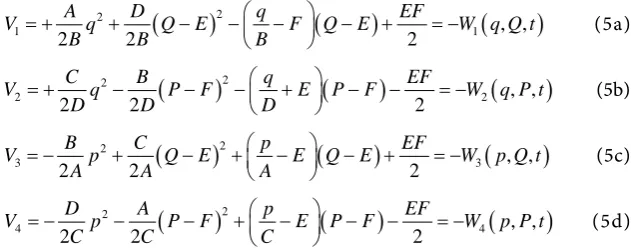
We listed four types of the generating functions in (5). From the theoretical and ex-perimental points of view, it sometimes happens that we cannot describe the affine transformation via one of them. For example, the affine transformation in (20) below has zero component in C=0. In that case, we cannot use (5d), but the other ones are

[image:3.595.237.553.166.290.2]

available. The relationship between these eikonals (generating functions) is depicted in Figure 1. The functions at the ends of the arrows are related to each other by a Legen-dre transformation. For example, from the relation (6a), we obtain the variable Q in terms of q and P,

(

)

1

W D q

P Q E F

Q B B

∂

₄

= - W

₄

V2= V1- QP

V₄= V₂+ qp

V4= V3- QP

[image:4.595.249.499.66.192.2]

V₃= V₁+ qp

Figure 1. The eikonals (generating functions) are disposed on the corners of the square. The functions at the ends of arrows are related to each other by a Legendre transformation.

Corresponding to the canonical transformation in classical mechanics, the unitary transformation plays a central role in quantum mechanics. Analogous to the classical affine transformation (1), we define the quantum mechanical affine transformation as follows,

†

ˆ ˆ _ˆˆ _ˆ _ˆ

Q=T qT =Aq+Bp+E, (7a)

†

ˆ ˆ _ˆˆ _ˆ _ˆ

P=T pT =Cq+Dp+F, (7b)

where ∧

describes the q-number and _Tˆ_{is a unitary operator which generates the} af-fine transformation. Here, AD−BC=1 is also needed when the canonical

commuta-tion relacommuta-tions

[ ]

_{q p}_{ˆ ˆ}_, =__{Q P}ˆ ˆ_, _=_i_{are satisfied.}

To obtain the unitary operator _Tˆ_{, we introduce two operators. One is the} displace-ment operator _Dˆ_,

[

]

ˆ _exp _ˆ _ˆ

D= −iEp+iFq (8)

which generates the displacements in position and momentum, †

ˆ _ˆˆ _ˆ

D qD= +q E, (9a)

†

ˆ _ˆ ˆ _ˆ

D pD= +p F. (9b)

The other one is the unitary transformation _Uˆ_,

2 2

ˆ ˆ ˆ ˆ ˆ ˆ

ˆ _exp _,

2 2 2

p qp pq q

U= −iα +β + +γ 

 

  (10)

which generates the ABCD-transformation [9] †

ˆ _ˆ ˆ _ˆ _ˆ

U qU = Aq+Bp, (11a)

†

ˆ ˆ ˆ ˆ

U pU =Cp+Dp, (11b)

where

cosh sinh sinh

sinh cosh sinh

A B

C D

β α

γ β

 _{∆ +} _∆ _∆ 

 

 _{= } ∆ ∆ _

 

  _ ₋ _∆ _{∆ −} _∆_

 ∆ ∆ 

, (12)

(5)

cosh cos sinh sin sinh

,

sin sinh cosh cos sinh

A B

C D

ξ θ ξ θ ξ

θ ξ ξ θ ξ

+

  ₌ 

   ₋ 

    (13)

then _Uˆ _{describes the squeezed operator}_[10]_.

We consider the unitary operator _Tˆ_{, which generates the quantum affine} transfor-mation (7), as a product of _Dˆ_and _Uˆ _,

ˆ ˆ ˆ

T =DU . (14)

Indeed, we obtain

(

)

† † † †

ˆ ˆ _ˆˆ ˆ ˆ _ˆˆ ˆ ˆ _ˆ ˆ _ˆ _ˆ

Q=T qT =U D qDU =U q+E U= Aq+Bp+E, (15a)

(

)

† † † †

ˆ ˆ _ˆˆ ˆ ˆ _ˆˆ ˆ ˆ _ˆ ˆ _ˆ _ˆ

P=T pT =U D pDU =U p+F U =Cq+Dp+F, (15b)

which is the quantum mechanical affine transformation (7) as we expected.

Now, we calculate the kernel of the affine transformation. The kernel is just the tran-sition amplitude from the potran-sition q at an initial time to the potran-sition Q at a later time given by affine

(

_,

)

ˆ

Q q = Q T q

 . To obtain the kernel, we use the coordinate identity operator

∫

dq q′ ′ q′ =1 between the displacement operator Dˆ and the unitary

op-erator _Uˆ _:

ˆ ˆ ˆ _d ˆ ˆ

Q T q = Q DU q =

∫

q Q D q′ ′ q U q′ (16)

Using the formulae

ˆ _exp

2 i

D q = +q E _+iFq+ EF_

 , (17a)

ˆ _exp

2 i

D p = p+F _−iEp− EF_

 , (17b)

we obtain

(

)

ˆ _d ˆ _exp

2

ˆ _exp _.

2 i

Q T q q Q q E q U q iFq EF

i

Q E U q iF Q E EF

 

′ ′ ′ ′

= + _ + _

 

 

= − _ − + _

 

∫

(18)

Substituting the transition amplitude in terms of _Uˆ _[9]_{, we obtain the result:}

(

)

2

(

)

2

1

ˆ _exp

2π 2 2 2

A D q EF

Q T q i q Q E F Q E

iB B B B

    

= _− −_ − − +_ − _ − − __

 

 

 . (19)

We include the “irrelevant” constant phase factor which has often been neglected in the literature [11][12]. The function in the exponent is in the same form as that of the generating function (5a). For example, let us consider a particle with mass m, subjected to a constant external force f, moving from

(

q p,

)

to

(

Q P,

)

in time t. The exact

so-lution for this problem is described in the following, 2 1

2

0 1

t ft

Q q

m m

P p

ft

 

  _ __{  } _

= +

  _ __{  } _

 

(6)

Substituting these parameters into (19), we obtain

(

)

2

(

)

2 3

ˆ _exp

2π 2 2 8

m m ft f t

Q T q i q Q q Q

it t m

[ ]

3 3

1 1

ˆ _exp _, _exp

2π 2π

Q T p iW p Q iV

A A

= _− _= _{, (22c)}

(

)

[ ]

4 4

1 1

ˆ _exp _, _exp

2π 2π

P T p iW p P iV

iC iC

− −

= _− _= _{, (22d)}

where the W’s in the exponentials are the generating functions (5) which generate the canonical transformation (1).

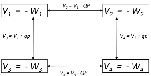
It is worth commenting here that it is well known in classical mechanics [8] that the generating functions (5) are related to each other by a Legendre transformation (Figure 1), whereas the kernels (22) are related to each other by a Fourier transformation. These relations are depicted in Figure 2.

4. Wavization of Gabor Function

Quantum mechanics is obtained by the “quantization” of classical mechanics. Similarly, physical optics is constructed by the “wavization” of geometrical optics [3] [6]. The famous example is that of Fraunhofer diffraction obtained by wavization of a plain wave. Let us consider the Gabor function [6][14];

(

)

1 4

2 0

0 0

2 2

1 1

exp

2

π 2

q

q Gabor ip q q q

σ σ

   

 

=_ _ _ _ − _− − _

     , (23)

where p0 is the wave number and qˆ =q0 is the center of this wave packet. The

<

_𝑄

|

_T�

|

_𝑞

>

<

𝑃

|

T�

|

𝑞

>

[image:6.595.254.495.560.677.2]

<

_𝑄

|

_T�

|

_𝑝

>

<

𝑃

|

T�

|

𝑝

>

(7)

width is obtained from

2 2

ˆ ˆ

2

q q q σ

∆ = − = . (24)

To make the calculation easier, this wave packet (23) can be rewritten in the form, 2

1 4 2 2

2 2 1 2 exp 2 2 π 2 z

q z z

q Gabor q

σ

σ σ

 

 

=_ _ − + − − 

  _ _, (25)

with 0

0 1

2 q

z i pσ

σ

 

= _ + _

 . Note that when σ =1, it gives the position-representation

of the coherent state wave function q z . It is also worth writing down the Fourier

transformation of (23) and (25),

(

)

1 4 2 2 2 0 0 0 exp

π 2 2

p

p Gabor =σ  −iq _p− _−σ p−p 

   , (26)

1 4 2

2 2 2

2

exp 2

π 2 2 2

z z

p i zp

σ  σ _σ 

 

=_ _ − − + − 

 

  _ _. (27)

Using this expression, we obtain pˆ =p0 and the width 2

2 1

ˆ ˆ

2

p p p

σ

∆ = − = _{. (28)}

This result with (24) gives

1 2

q p

∆ ⋅ ∆ = _{, (29)}

that is, the Gabor function satisfies the minimum uncertainty relation.

We obtain the affine transformation of the Gabor wave packet by using the kernel (22),

(

)

(

)

2

1 4 * 2

2

2 2 2

ˆ _d ˆ

1 2

exp ,

2 2 2

π 2

Q T Gabor q Q T q q Gabor

z

H z G z EF

Q E iF Q E i

G G

G G σ

σ σ =       =_ _ − − +_ + _ − − − +   _ _   

∫

(30) and

(

)

(

)

1 4 2

2 2 * 2

2 2

ˆ _d ˆ _d ˆ

2

exp ,

2 2 2 2

π

P T Gabor q P T q q Gabor p P T p p Gabor

z

G z H z EF

P F i E P F i

H H H

H

σ σ σ

= =  _ _    =  − − − _ + _ − + − −         

∫

(31)

where we introduce two complex variables,

2

B

G A i

σ

= + , (32a)

2

H= −D iσ C. (32b)

(8)

(

)

{

}

2 2

0 0

2 2

1 1

ˆ _exp

π

Q T Gabor Q Aq Bp E

G G

σ σ

 

= − − + + 

 

 , (33a)

(

)

{

}

2 2

0 0

2 2

ˆ _exp

π

P T Gabor P Cq Dp F

H H

σ  σ 

= − − + + 

 

 . (33b)

The center of the Gabor function propagates along the affine transformation (1). From these Equation (33), we obtain the variances

2 2

ˆ ˆ

2

Q Q Q σ G

∆ = − = _{, (34a)}

2 2

ˆ ˆ

2 H

P P P

σ

∆ = − = _{, (34b)}

and the uncertainty relation

(

)

2

2 2 4 2

4

1 1

2 2

B

Q P G H A D σ C

σ

 

∆ ⋅ ∆ = ⋅ = _ + _ +

  . (35)

Since the only constraint for the parameters

(

A B C D, , ,

)

is AD−BC=1, these

parameters have time dependency. So, these results (34) and (35), show the time de-velopment of the variances and the uncertainty relation of the Gabor function.

Let us show two examples here. As we saw in (25), the Gabor function with σ =1

signifies a coherent state. So, using (13) as

(

A B C D, , ,

)

, (35) becomes

(

)

2

1

1 sinh 2 sin 2

Q P ξ θ

∆ ⋅ ∆ = + _{, (36)}

which coincides with the uncertainty relation of the squeezed state [10]. The other ex-ample is where we use (20), then (35) becomes

2

4 2

1 1 2

t

Q P

m

σ

∆ ⋅ ∆ = + _{, (37)}

which coincides with the uncertainty relation [15] of the spreading of the Gaussian wave packet in time.

5. Affine Transformation of the Wigner Function

The Wigner function [16]-[18] is widely used in studying optics and the correspon-dence between classical and quantum mechanics [6][7]. The Wigner function for any wave function ψ is defined by

(

,

)

d e

2 2

iuP u u

f Q P =

∫

u Q− ψ ψ Q+ . (38)

When we take a Gabor function (23) for any wave function ψ = Gabor , the Wigner

function (38) becomes

(

)

(

)

2 ₂

(

)

2

0 0

2 1

, 2 exp

G

f Q P Q q σ P p

σ

 

= _− − − − _

(9)

Now we apply the unitary operator _Tˆ_{to any wave function;} _ψ _→_Tˆ_ψ _{. We} ob-tain the affine transformation of the Wigner function,

(

)

_ˆ _ˆ†

, d e

2 2

affine iuP u u

f Q P =

∫

u Q− T ψ ψ T Q+ . (40)

To cast the right hand side, we use the coordinate identity operator

∫

dx x x =1 twice,

†

ˆ ˆ

d d d e

2 2

iuP u u

u x x′ Q− T x xψ ψ x′ x T Q′ +

∫

. (41)

Substituting the kernel (22a) into (41) and integrating over u, we obtain

(

)

(

)

(

)

2 2

d d

exp

2π 2

2π ,

2

x x A Q E

x x i x x i x x

B B B

D Q E x x

P F

B B

ψ ψ

δ

′ _′  ₋ _′ ₋ − ₋ _′

 

 

−

 + ′

×  − − + 

 

∫

(42)

where δ

( )

z is a delta function of z. Changing the variables u= −x x′ and

2

x x

v= + ′,

we obtain

(

)

(

)

(

)

d d

exp

2π 2 2

2π ,

u v u u A Q E

v v i uv i u

B B B

B B P F D Q E v

ψ ψ

δ

−

 

+ − _ − _

 

× − − − +

∫

₍₄₃₎

where we use the formula

( )

1

( )

ax a x

δ ₌ −δ _{. Integrating over}

v, we obtain

(

)

{ ( ) ( )}

(

)

(

)

(

)

(

)

, d e

2 2

iu A P F C Q E affine

f Q P u

u u

D Q E B P F ψ ψ D Q E B P F

− − −

=

× − − − − − − − +

∫

, (44)

where we use AD−BC=1 and change the variable u→ −u. This is the affine

trans-formation of the Wigner function which is a generalization of (38) and can be applied to any wave function ψ _{and to any affine transformation with the condition AD –}

BC = 1. Equation (44) shows that the ABCD-part describes the area-preserving distor-tion, and the E, F-part describes the displacement in phase space. It is permissible for any affine transformation to have time dependency, so we are able to investigate the dynamic properties of the Wigner function in phase space.

As an example of a wave function ψ , we take a Gabor function. Substituting the Gabor function (23) into (44) and integrating over u, we obtain

(

)

(

)

(

)

{

}

2 ₂

{

(

)

(

)

}

2

0 0

2 ,

1 2 exp

affine G

f Q P

D Q E B P F q σ A P F C Q E p

σ

 

= _− − − − − − − − − − _

 

. (45)

(10)

(

)

2

d _ˆ

, 2π

affine G P

f Q P = Q T Gabor

∫

, (46a)

(

)

2

d _ˆ

, 2π

affine G Q

f Q P = P T Gabor

∫

, (46b)

which is the correct character of the Wigner function.

6. Summary

We have developed the mathematical properties of an affine transformation from the optical and mechanical points of view. The kernels of the affine transformation were clearly derived and comprise the eikonals (generating functions) which generated the affine transformation in optics (mechanics).

Using the kernel, we discussed the wavization of the Gabor function. The Gabor function has a Gaussian profile and is symmetric in position and momentum. We found the time development of the uncertainty relation, according to the affine trans-formation.

We also discussed the affine transformation of the Wigner function and showed not only the distortion but also the dynamic movement of the Wigner function in phase space.

References

[1] Hecht, E. and Zajac, A. (1974) Optics. Addison-Wesley, Boston.

[2] Mickelson, A.R. (1992) Physical Optics. Van Nostrand Reinhold, New York. http://dx.doi.org/10.1007/978-1-4615-3530-0

[3] Guillemin, V. and Sternberg, S. (1984) Symplectic Technique in Physics. Cambridge. [4] Moshinsky, M. and Quesne, C. (1971) Journal of Mathematical Physics, 12, 1772.

http://dx.doi.org/10.1063/1.1665805

[5] Boon, M.H. and Seligman, T.H. (1973) Journal of Mathematical Physics, 14, 1224. http://dx.doi.org/10.1063/1.1666470

[6] Torre, A. (2005) Linear Ray and Wave Optics in Phase Space. Elsevier, Amsterdam. [7] Ozaktas, H.M., Zalevsky, Z. and Kutay, M.A. (2001) The Fractional Fourier

Transforma-tion. John Wiley & Sons, Hoboken.

[8] Goldstein, H. (1950) Classical Mechanics. Addison-Wesley, Boston. [9] Ogura, A. (2009) Journal of Physics, B42, 145504.

http://dx.doi.org/10.1088/0953-4075/42/14/145504

[10] Stoler, D. (1970) Physical Review D, 1, 3217. http://dx.doi.org/10.1103/PhysRevD.1.3217 [11] Abe, S. and Sheridan, J.T. (1994) Journal of Physics, A27, 4179.

http://dx.doi.org/10.1088/0305-4470/27/12/023 [12] Cai, L.Z. (2000) Optics Communications 185, 271-276.

http://dx.doi.org/10.1016/S0030-4018(00)01005-1

[13] Feynman, R.P. and Hibbs, A.R. (1965) Quantum Mechanics and Path Integral. McGraw- Hill Inc., Boston.

[14] Gabor, D. (1946) J. of the IEE, 93, 429.

(11)

[16] Wigner, E.P. (1932) Physical Review, 40, 749. http://dx.doi.org/10.1103/PhysRev.40.749 [17] Kim, Y.S. and Wigner, E.P. (1990) American Journal of Physics, 58, 439.

http://dx.doi.org/10.1119/1.16475

[18] Hillery, M., O’connell, R.F., Scully, M.O. and Wigner, E.P. (1984) Physics Reports, 106, 121-167. http://dx.doi.org/10.1016/0370-1573(84)90160-1

Submit or recommend next manuscript to SCIRP and we will provide best service for you:

Accepting pre-submission inquiries through Email, Facebook, LinkedIn, Twitter, etc. A wide selection of journals (inclusive of 9 subjects, more than 200 journals)

Providing 24-hour high-quality service User-friendly online submission system Fair and swift peer-review system

Efficient typesetting and proofreading procedure

Display of the result of downloads and visits, as well as the number of cited articles Maximum dissemination of your research work