Munich Personal RePEc Archive
Exploring environmental urban policies:
a methodological proposal to build a
composite indicator measuring urban
environmental virtuosity
Ercolano, Salvatore and Romano, Oriana
Second University of Naples, University of Naples L’Orientale
31 January 2011
Online at
https://mpra.ub.uni-muenchen.de/29230/
Exploring environmental urban policies: a methodological proposal to build a composite indicator measuring Urban Environmental Virtuosity
Salvatore Ercolano
Department of Law and Economics
Second University of Naples
Oriana Romano
Department of Social Sciences
University of Naples L’Orientale
Abstract
Synthesizing the complex phenomenon of “environment” into a single indicator could leads to a loss of information, which inhibit his use as a reference for the resolution of several issues such as, for example, the allocation of resources. On the other hand it allows to represent the overall environmental performance of cities and to highlight relationships between different sectors. We consider “process oriented” variables instead of aggregated and “outcome oriented” ones, generally used to measure environmental sustainability strictu sensu. In this sense we refers specifically to the concept of “environmental virtuosity”, that allows to rank statistical units (i.e. Italian main municipalities), considering their policy efforts for improving urban environmental quality. Generally an indicator of environmental quality should combine partial information to summarize the main subject. This paper proposes to measure urban environmental virtuosity by multivariate analysis, following OECD (2008) procedure. This methodology will try to overcome the main methodological issues in building up indicators, consisting in the choice of weights and in the common practice of simply adding sub-indicators.
1. Object of the research paper
In order to manage resources in a sustainably way and to ensure an appropriate level of environmental quality, decision makers need to: identify objectives to be pursued; choose the most suitable tools (policies, persuasive and dissuasive actions, command and control, environmental taxation) to achieve that goals, then monitor and evaluate results. It would be suitable to take decisions and to evaluate responses by referring to a system of environmental indicators, by which immediately and easily to identify actions to be sorted out, so to improve the state of the environment at local level.
“outcome oriented” ones, generally used to measure environmental sustainability strictu sensu, because they are purely physical parameters.
Based on these considerations, this paper proposes to measure urban environmental virtuosity by multivariate analysis, following OECD (2008) procedure. First, we will categorize statistical units by cluster analysis as a function of a set of indicators, considered explanatory of the phenomenon; then we will determine a composite indicator of environmental virtuosity at local level by factor analysis.
By cluster analysis we will reduce the size of data to be analyzed: from the total number of statistical units to the number of clusters, providing a description of the statistical units, by features as common elements of the same group, but not common for the others. Cluster analysis results will be compared with an indicator of environmental virtuosity, as well as to verify the consistency.
Synthesizing the complex phenomenon of “environment” into a single indicator could leads to a loss of information, which inhibit his use as a reference for the resolution of several issues such as, for example, the allocation of resources. On the other hand it allows to represent the overall environmental performance of cities and to highlight relationships between different sectors.
Conscious of the limits of composite indicators in describing a phenomenon, our purpose is to put in practice a methodology illustrated by OECD by which to obtain an indicator of virtuosity, rather than sustainability one. This methodology will try to overcome the main methodological issues in building up indicators, consisting in the choice of weights and in the common practice of simply adding sub-indicators.
2. Backgrounds on Urban environmental indicators
Local level has always been a starting point for the implementation of policies related to the achievement of environmental sustainability; moreover international organizations (UN: Rio de Janeiro Conference in 1992, Habitat Istanbul Conference in 1996; OECD: Cities for Citizens. Improving Metropolitan Governance, 2000) and European Union (Aalborg Charter, 1994, Framework Programmes) strongly promote urban sustainability. Currently there are several indicators measuring urban environmental sustainability (Singh RK et al. 2009), developed from nineties; some examples are provided: Stanners, D., Bourdeau, P., (1991) define 3 categories of indicators, considering 55 sub indicators: 1) Indicators of urban patterns, as the sum of Urban population; Urban land cover; Derelict areas; Urban renewal areas; Urban mobility; Commuting patterns; traffic volumes; 2) Indicators of urban flows, considering Water: water consumption, Wastewater; Energy; Materials and products (transportation of goods); Waste; 3) Indicators of urban environmental quality: Quality of water; Quality of air; Acoustic quality ; Traffic safety (fatalities and casualties from traffic accidents); Housing quality; Accessibility of green space; Quality of urban wildlife (number of bird species).
Indicators on urban environmental quality by OECD (1993) are divided in three types of indicators: Environmental pressures (urban air emissions SOx, NOx, VOC, traffic density, degree of urbanisation), Environmental conditions (exposure of population to air pollutants, noise, ambient water conditions in urban areas, concentration of air pollutants), societal responses (changes in green space as a percentage of total urban area/total urban population, regulations on emissions and noise levels for new cars, expenditure on water treatment and noise abatement).
Legambiente (1994) in “Urban Ecosystem” report measures urban sustainability based on 25 indicators of environmental quality, representative of factors of pressure, quality of environment, capacity of response and environmental management. Data collection is based on interviews submitted periodically to provincial municipalities and on the basis of other statistical sources. Indicators cover all major environmental components: air, water, waste, energy and allow to make a ranking of the cities analyzed.
functional composite indicator, by the arithmetic average of 22 sub-indicators. (Saisana M., Tarantola S., 2002).
Environmental statistics of Helsinki (1998) is a report that provides a study of the impact of human activities on the environment. Environmental indicators are: City structure, Pollution load from urban activities (traffic, energy consumption of traffic, emissions from traffic, traffic noise, accidents, jobs and industry, energy production and distribution system, energy consumption, emissions from energy production and manufacturing, waste from energy production and beneficial use of this waste, water provision, drinking water quality, waste water load, waste and its management), State of the environment (total emissions by source, carbon dioxide, climate change, air quality, acid deposition of sulphur and nitrogen, water quality), Biodiversity (plants, birds).
European Common Indicators (ECI), by Expert Group on Urban DG Environment of European Commission (Rapporto Ambiente Italia, 2003), are taken on basis of data provided by interviews to different urban areas. Indicators put highlights on the possible lack of facilities services, allow to increase awareness on issues of environmental management, stimulate interest in development of sustainable products, etc.
Istat (2009), in the “Environmental data in the cities” report ranks provincial municipalities looking at a synthetic indicator of eco-friendly, calculated from the average of the standardized indicators. These are defined using DPSIR method (Istat, 2009). Data collection is carried out periodically since 2000. It consists of the compilation online by public and private urban bodies of seven questionnaires, each of which relates to a specific environmental theme.
Considering this few examples of urban environmental indicators, we set out some remarks about the choice of data and on methodology used to calculate a composite indicator: two issue that we will try to handle in this paper.
The choice of data as sub indicators is crucial for a correct definition of a certain phenomenon: obviously the same phenomenon could be represented by several indicators, considering the availability of data of statistical units considered. This means that even if indicators have the same purpose, for instance measuring environmental quality of cities, they will be different from each others and not comparable. The choice of sub indicators and the availability of data are not the only issue in defining composite indicators. There is also a methodological problem consisting in assigning, by a personal judgment, weights and in adding sub indicators in order to find out a composite one. As OECD (2008) claims, in the building up of a composite indicators, there are several suitable techniques to be applied, as multivariate analysis, able to overcome that issue and to provide a more efficient indicator from a structural point of view.
3. Measuring Urban Environmental Virtuosity (UEV): data and methodology
In the following paragraph we attempt to identify a methodological strategy to overcome the problems concerning in the composite indicators by means of a multivariate approach; the empirical test will be performed on the Italian urban contest.
More specifically, the analysis involves 111 provincial municipalities, according to the availability of data on environmental subjects provided by ISTAT. Municipalities considered covers capitals of 6.6% of Italian surface and the 29.5% of the total population of the country (about 17 million people)1.
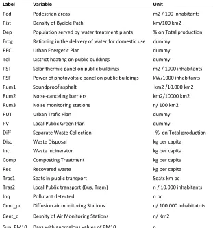
For the variables choice we try to identify indicators directly related to policy choice for each municipality in the environmental domain (see tab. 1); more specifically the selected indicators concern all the available responses defined by local public body in order to improve environmental quality, regardless of specific morphological characteristics.
Policy choices in environmental domain can be divided in 6 sub-domains; for each one we analyze several indicators as follow:
• Transport (Pedestrian areas, Bycicle path, Urban Trafic Plan, Seats in public tran sport, Local Public transport)
• Waste (Separate Waste Collection, Waste Disposal, Waste Incinerator, Composting Treatment, Recovered waste)
• Water (Water treatment plants, Rationing water for domestic use)
• Energy (Urban Energetic Plan, District heating on public buildings, Solar thermic panel on public buildings, Power of photovoltaic panel on public buildings)
• Green2 (Green Local Public Plan)
• Urban environmental (Soundproof asphalt, Noise-canceling barriers, Noise monitoring stations, Pollutant detected, Diffusion air monitoring Stations, Density of Air Monitoring Stations, Days with anomalous values of PM10)
The empirical strategy to define the different behavior of municipalities in term of virtuosity will be carried out by two approaches. First of all a cluster analysis will be provided: it allows to classify statistical units, highlighting features as common elements of the same group and that make each group distinct from the others. The main advantage is to synthesize the phenomenon into categories characterized by the presence or absence of certain relevant dimensions and to reduce the size of data: from the total number of statistical units to the number of clusters. The grouping is done by the method of hierarchical classification.
Then, using factorial analysis techniques it will be possible to identify a urban environmental virtuosity index (UEVI), overcoming the problem of choosing weights as currently happens for the definition of composite indicators (OECD 2008).
Variables selected for each sub domain are analyzed by means of PCA with varimax rotation (Linting et al., 2007; Svedin, 2009).
As is well known, PCA permits to identify a certain number of latent factors representing the data and their variance. Each one of them depends on a set of coefficients (loadings) that measure the correlation between the original variables and the latent factor.
Following various practices, factors (subdomains) may be extracted in an optimal number in order to represent the original data minimizing the loss of variance in the dataset. Varimax rotation may be used to minimize the number of indicators that have a high loading on the same factor and so to obtain a “simpler structure” of the factors that helps their interpretation (OECD, 2008). As well known, the eigenvalue represents the explained variance of each factor. The first one has the maximum variance (fig. 1), so it could represents a good synthesis of the phenomenon; on the other hand, each factor is characterized by the different contributions of the original values (see coefficient in tab 2). To merge different information, captured by each factor, we will try to build a composite index for Urban Enveiromental Virtuosity following the methodology proposed by the Oecd (2008)and few papers (Nicoletti et al, 2000; Coco and Russo, 2006; Ercolano and Gaeta, 2010, De Simone et al 2010). For each j-th municipality the index value is calculated as follows:
2 For green domain in a first analysis we had used other variables (such as gree avaibility and green density); but these
Where:
R represents the UEV indicators for e
x represents the original variables
α, β and ω rapresent the coordinate
represents the eigenvalue associa
The approach followed consists in variance that is explained by the fac factor [subdomain] was weighted ac the dataset [in the domain]” [Nicolet
4. First results
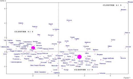
Performing cluster analysis, by mean minimize the intra-cluster inertia procedure, we obtain 3 cluster as rep the municipalities and the centre o analysis in table 3. On the top we bottom part we find the variables absence (negative t-value). The first effective policy in the waste (crucial and negative T Vale for waste dispo good value too; but it seems not to h
Second cluster is composed just by 2 axis extracted by the analysis; it is ch policy, such as soundproof asphalt, n solar thermic panel on public building
Third cluster, composed by 50 mu policies, especially in waste sector (s Value for Waste disposal in land characteristics for this group are: rati days with anomalous values of PM1 control of the scarcity of water reso size of municipalities.
The main strengths of cluster analy structure of the data set, but it is information held in the original var variables that synthesize the original of different variables, so we try to
for each j-th municipalities
nates of each i-th original variables on extracted fact
ociated to each excracted factor
in “ weighting each detailed indicator according to factor it is associated to (i.e. the normalised square d according to its contribution to the portion of the oletti et al, 2000].
eans of a parti-decla procedure, we are able to ge tia (variability) and maximize the inter-cluster i s reported in tab 2. We report also the factorial plan re of the clusters (see fig. 2) and the characteriz we find the main municipality represented in each les that characterize the cluster for their presenc first one is characterized by “positive” and “negat cial variables show positive high T-value for all sep isposal in landfill); sustainable mobility policies and to have a good quality of the air.
by 2 municipalities that shows the higher coordinat is characterized by positive and specific aspects, re
lt, noise changeling barriers, noise monitoring statio lding and bicycle path.
municipalities, is characterized by the lack of ef r (see high negative T Values for separate waste co landfill), but also in energy and sustainable m rationing in the delivery of water for domestic use, PM10. Results of the former variables could be in esources, while the latter could be given from the
nalysis is to offer a way to group countries giving is purely a descriptive tool and it is not able to m variables. As we have explained above, factorial
inal selected indicators, but in each extracted facto to merge all the factors by the methodology, exp
factors
g to the proportion of its uared loading), while each f the explained variance in
o generate a partition that er inertia. Following this an with the projection of terization of first factorial each cluster, while in the sence (positive t-value) or gative” aspects; it has an separate waste collection and energy sectors show
inate on the two factorial , related to infrastructural tation, district heating and
f effective environmental e collection and positive T mobility ones. Positive se, pollutant detected and e influenced by a political the average medium-small
paragraph. This is the main attempt of our composite indicator – Urban Environmental Virtuosity Index (UEVI) – building up following the reported OECD methodology.
In tab 4 we report the ranking achieved by each municipality using UEVI. At first glance in the top position we find north municipalities (except two municipalities of Sardinia region). This is confirmed by aggregated analysis, defined considering South, North and Centre (see tab 5) and the regional level (see tab 6 and fig. 3).
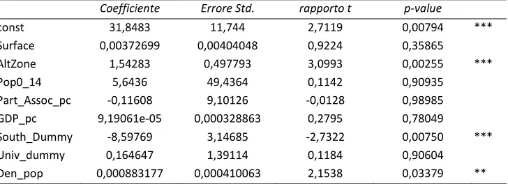
These results are consistent with a preliminary OLS regression results (see tab 7, 8). Considering some crucial variables, in affecting Environmental policy choices, such as social-demographics, spatial, educational and cultural ones, we find out that UEVI is positively affected by two variables: altimetric zone and population density. On the other hand it is negatively influenced by the localization of municipalities in the south of Italy. UEVI seems not to be affected by economic, cultural-educational variables.
5. Conclusions
Currently a crucial issue for decision makers and citizens is to measure what we have called “environmental virtuosity”, that implies to verify if actions to improve environmental quality in urban contexts are taken by local public bodies and their level of effectiveness in achieving certain goals. The aim of the first part of the analysis has been to provide a summary of statistical units, in order to consider the level of virtuosity provided by several municipalities, while the second part has provided a ranking of them considering an indicator of environmental performance, able to measure the efficiency of instruments used by decision-makers, obtained by multivariate approach. Even if environmental composite indicators at urban level already exist, their effectiveness depends on the choice of data (sub-indicators) and of methodology applied to built them. In order to overcome methodological issues arisen from weighting and adding them, we construct UEVI by using factorial analysis. It allows to merge all the different information held in the original variables and to better represent a complex phenomenon as the efficacy environmental choices made by decision makers at local level is. Transport, waste, energy, water and other key sectors by a social and economical point of view can be managed in a sustainable way, but the level of environmental quality achieved by municipalities need to be measured. It could be helpful to understand which of these sectors need to be “environmentally” improved. Obviously this level of virtuosity could be affected by other external variables and not only by political choices. Our ranking shows a strong difference among municipalities situated in the north and in the south of Italy, but differently as it can be imagined, as OLS results show, it do not depends from cultural and educational variables.
Bibliography
COCO ., RUSSO M. (2006), Using CATPCA to evaluate market regulation, in Zani S. et al (ed. by) Data Analysis Classification and the Forward search, Springer, pp.369-376
De Simone E., Ercolano S., Gaeta G.L., (2010), Exploring Capitalism(s), EAEPE conference Ercolano S., Gaeta G.L., (2010), Reassessing the power of purse, DYSES conference
Isla M. ( 1996), A review of the urban indicators experience and a proposal to overcome current situation. The application to the municipalities of the Barcelona province, Departament d’Economía Aplicada Autonomous University of Barcelona
Istat (2009), Indicatori ambientali urbani, Rapporto Istat
Legambiente (1994), Ecosistema urbano: Rapporto sulla qualità ambientale dei comuni capoluogo di provincia, http://www.legambiente.eu/documenti/1989-1996/ecosistemaUrbano1994.pdf
NICOLETTI G., SCARPETTA S. AND BOYLAUD O. (2000), Summary indicators of product market regulation with an extension to employment protection legislation, OECD Economics department working papers No. 226
OECD 1993 core set of indicators for environmental performance reviews, a synthesis report by the Group on the State of the Environment, Environmental monographs n.83.
OECD (2008) Handbook on Constructing Composite Indicators: Methodology and User Guide, OECD Publishing
Rapporto di Ambiente Italia (2003), Verso un quadro della sostenibilità a livello locale - Indicatori comuni europei (ICE), Roma.
Rostirolla P. (1998), La fattibilità economico-finanziaria: metodi e applicazioni, Liguori editore, Napoli.
Saisana M., Tarantola S., 2002, State-of-the-art Report on Current Methodologies and Practices for Composite Indicator Development, EUR Report 20408 EN, European Commission, JRC-IPSC, Italy. Singh R., K., Murty H.R., Gupta S.K., Dikshit A.K., (2009), An overview of sustainability assessment methodologies, Ecological Indicators, pp. 189-212
Stanners, D., Bourdeau, P., Europe’s environment: the Dobris assessment, European Environment Agency, Copenhagen 1991.
Appendix: tables and graphics
tab. 1: considered variables
Label Variable Unit
Ped Pedestrian areas m2 / 100 inhabitants
Pist Density of Bycicle Path km/100 km2
Dep Population served by water treatment plants % on Total production
Erog Rationing in the delivery of water for domestic use dummy
PEC Urban Energetic Plan dummy
Tel District heating on public buildings dummy
PST Solar thermic panel on public buildings m2 / 1000 inhabitants
PSF Power of photovoltaic panel on public buildings kW/1000 inhabitants
Rum1 Soundproof asphalt km2 /10.000 km2
Rum2 Noise-canceling barriers km2/10000 km2
Rum3 Noise monitoring stations n/ 100 km2
PUT Urban Trafic Plan dummy
PV Local Public Green Plan dummy
Diff Separate Waste Collection % on Total production
Disc Waste Disposal kg per capita
Inc Waste Incinerator kg per capita
Comp Composting Treatment kg per capita
Rec Recovered waste kg per capita
Tras1 Seats in public transport Seats km pc
Tras2 Local Public transport (Bus, Tram) n / 10.000 inhabitants
Inq Pollutant detected n pc
Cent_pc Diffusion air monitoring Stations n/ 100.000 inhabitatnts
Cent_d Desnity of Air Monitoring Stations n/ Km2
[image:9.595.142.453.143.475.2]Sup_PM10 Days with anomalous values of PM10 n
Component
1 2 3 4 5 6 7 8 9
Ped ,059 -,249 ,602 ,382 ,066 -,134 ,178 -,006 ,196
Pist ,480 ,302 -,011 ,356 ,231 ,142 ,085 ,398 -,067
Dep ,102 ,022 -,052 -,052 -,025 ,759 ,193 -,060 ,050
Erog -,218 -,028 -,041 -,002 -,025 -,132 -,745 -,502 -,058
PEC ,255 ,030 ,555 -,099 -,451 -,088 -,243 -,155 ,057
Tel ,275 ,499 ,224 ,306 ,101 ,332 -,261 ,283 -,230
PST -,068 ,179 -,090 ,130 -,047 ,061 ,461 -,155 -,290
PSF -,300 -,150 -,207 -,141 -,035 ,541 ,076 -,087 ,492
Rum1 ,155 ,780 ,220 -,088 -,075 -,005 ,047 ,009 ,256
Rum2 ,030 ,898 ,052 ,041 ,062 ,012 ,148 ,011 -,060
Rum3 -,224 ,806 -,045 ,038 ,000 -,238 ,034 -,155 -,063
PUT ,255 ,066 ,141 ,142 ,133 ,021 ,731 -,244 -,109
PV ,017 ,102 ,020 ,226 -,120 -,030 -,219 ,076 ,835
Diff ,876 -,032 -,003 ,357 -,005 -,003 ,100 ,017 -,013
Disc -,485 -,034 -,012 -,814 ,111 ,037 -,131 ,029 ,002
Inc ,080 ,037 ,030 ,909 -,100 -,126 ,079 ,081 ,159
Comp ,847 ,009 -,120 -,013 -,031 -,155 ,112 ,022 ,046
Rec ,555 -,147 ,109 ,393 -,071 ,267 ,099 ,390 -,172
Tras1 -,082 ,096 ,885 -,006 ,019 -,167 ,084 ,054 -,021
Tras2 -,128 ,274 ,813 -,020 ,176 ,085 -,031 ,078 -,107
Inq ,358 ,235 ,172 ,068 ,082 -,674 ,224 ,059 ,301
Cent_pc ,103 -,153 ,013 -,026 ,863 -,026 -,025 -,052 -,016
Cent_d -,102 ,224 ,143 -,163 ,812 -,075 ,078 -,087 -,091
Sup_PM10
Tab. 2: Cluster Analysis results
Cluster 1 / 3 Count: 55 Cluster 2 / 3 Count: 2 Cluster 3 / 3 Count: 50
Rank Case identifier Rank Case identifier Rank Case identifier
1 Pavia 1 Bolzano 1 Brindisi
2 Rimini 2 Bologna 2 Salerno
3 Livorno 3 Chieti
4 Lecco 4 Messina
5 Verona 5 Lecce
6 Belluno 6 Catanzaro
7 Pordenone 7 Campobasso
8 Alessandria 8 Agrigento
9 Firenze 9 Avellino
10 Pisa 10 Taranto
Characteristic
variables Test-value
Characteristic
variables Test-value
Characteristic
variables Test-value
Diff 7,99 Rum1 7,10 Disc 7,57
Rec 7,47 Rum3 6,86 Erog 4,78
Pist 5,38 Rum2 6,29
Inc 5,27 Tel 3,52 Ped -2,68
Comp 5,25 Pist 2,85 PEC -2,84
Sup_PM10 4,92 PST 2,57 Tel -3,34
Inq 3,28 Inq -3,81
Ped 2,69 Sup_PM10 -4,92
PEC 2,64 Comp -5,36
Tel 2,38 Inc -5,72
Pist -6,16
Rum3 -2,46 Rec -7,41
Erog -4,58 Diff -8,17
Fig. 2: factorial plan
Tab. 3: characterization of first factorial axis
Variable label Coordinate
Disc -0,75
Erog -0,53
PSF -0,27
Cent_pc -0,14
M I D D L E A R E A
Sup_PM10 0,54
Inq 0,54
Inc 0,62
Diff 0,71
Rec 0,72
Tab. 4: UEVI ranking
Rank Municipality UEVI Rank Municipality UEVI Rank Municipality UEVI
1 Venezia 67,36295 37 Bergamo 41,63349 73 Trieste 34,5864
2 Massa 58,58535 38 Verona 41,5967 74 Chieti 34,41079
3 Rimini 55,04188 39 Treviso 41,06623 75 Crotone 34,2527
4 Ravenna 54,25123 40 Ancona 40,84767 76 Imperia 34,05143
5 Brescia 54,04574 41 Parma 40,71088 77 Genova 33,92952
6 Reggio Nell'Emilia 51,59164 42 Cuneo 40,50554 78 Viterbo 33,90423
7 Torino 51,53233 43 Bari 40,17672 79 L'Aquila 33,8009
8 Padova 51,52266 44 Pistoia 39,88983 80 Teramo 33,7053
9 Piacenza 50,72276 45 Bolzano 39,58984 81 Aosta 33,52266
10 Lucca 50,32711 46 Cagliari 39,52322 82 Messina 33,31803
11 Pisa 49,71646 47 Palermo 39,4171 83 Lecco 32,84916
12 Mantova 49,55781 48 Pescara 39,24076 84 Sassari 32,46104
13 Alessandria 49,29588 49 Oristano 39,06511 85 Rieti 32,17225
14 Prato 48,91584 50 Perugia 38,76533 86 Caltanissetta 31,93247
15 Cremona 48,6885 51 Napoli 38,74441 87 Caserta 31,89524
16 Forli' 48,4902 52 Sondrio 38,34939 88 Medio Campidano 31,8161
17 Pesaro 47,82155 53 Udine 38,33723 89 Cosenza 31,70531
18 Firenze 47,50523 54 Livorno 38,24346 90 Macerata 31,11444
19 Siracusa 47,37581 55 Brindisi 37,99002 91 Foggia 30,81768
20 Olbia-Tempio Pausania 46,9648 56 Taranto 37,78901 92 Reggio Di Calabria 30,67609
21 Rovigo 45,71611 57 Frosinone 37,61709 93 Avellino 30,67594
22 Verbania 45,66665 58 Como 37,52623 94 Carbonia Iglesias 30,31072
23 Vercelli 45,48692 59 Savona 37,39841 95 Gorizia 29,83578
24 Catania 45,21594 60 Lecce 37,32084 96 Catanzaro 29,36849
25 Ferrara 44,5399 61 Trento 37,14107 97 Nuoro 29,08717
26 Bologna 44,39222 62 La Spezia 37,02818 98 Benevento 28,76909
27 Modena 44,38738 63 Varese 37,00193 99 Ragusa 28,4285
28 Roma 44,38128 64 Arezzo 36,46094 100 Campobasso 27,55304
29 Vicenza 44,13685 65 Latina 36,34615 101 Enna 27,4824
30 Siena 43,60463 66 Pordenone 36,33895 102 Belluno 27,44757
31 Grosseto 43,52498 67 Salerno 36,17448 103 Trapani 27,02759
32 Terni 43,52389 68 Agrigento 35,46521 104 Potenza 26,70072
33 Pavia 43,05946 69 Novara 35,38496 105 Matera 25,89601
34 Milano 42,33893 70 Biella 34,94104 106 Ogliastra 25,74042
35 Ascoli Piceno 42,19345 71 Vibo Valentia 34,82439 107 Isernia 25,23598
Tab. 5: Average UEVI for macro-zone
Geo Area Average Dev St
South 33,7088888 5,684656
North 42,3715595 7,806131
Centre 42,1648163 6,786676
Tab. 6: UEVI at regional level
Rank Region Average Dev.St
1 Emilia Romagna 48,2364543 4,998587
2 Toscana 45,6773823 6,675073
3 Veneto 45,5498677 12,08948
4 Lombardia 42,4418349 6,231189
5 Piemonte 42,186866 6,748531
6 Umbria 41,1446115 3,364814
7 Marche 40,4942751 6,944599
8 Trentino 38,3654544 1,731541
9 Lazio 36,8841991 4,693495
10 Puglia 36,8188551 3,530376
11 Liguria 35,6018836 1,867488
12 Abruzzo 35,2894393 2,652683
13 Friuli 34,7745909 3,631664
14 Sardegna 34,3710722 6,930788
15 Sicilia 33,5359057 6,352066
16 Valle d'Aosta 33,5226575 0
17 Campania 33,2518321 4,101246
18 Calabria 32,1653958 2,328063
19 Molise 26,3945102 1,638409
20 Basilicata 26,2983629 0,569017
Tab. 7 Label Surface AltZone Pop0_14 Part_Ass GDP_pc South_D Univ_du Den_pop
Tab. 8: First results
Coefficie
const 31,848
Surface 0,003726
AltZone 1,5428
Pop0_14 5,6436
Part_Assoc_pc -0,1160
GDP_pc 9,19061e
South_Dummy -8,5976
Univ_dummy 0,16464
[image:15.595.118.482.617.749.2]Den_pop 0,000883
Fig. 3: UEVI at regional level
7: Description of variables used in OLS regression
Description ace Municipality surface
one Atimetric zone of municipality
0_14 Population 0-14 (% of total population)
_Assoc_pc Index of parties and association
_pc Gross Domestic Product (current price)
h_Dummy South region
_dummy Presence of University institution
_pop Population Desnity
ults of OLS regression (dependent variable UEVI; R-squared 0,
ficiente Errore Std. rapporto t p-value
,8483 11,744 2,7119 0,00794
372699 0,00404048 0,9224 0,35865
4283 0,497793 3,0993 0,00255
6436 49,4364 0,1142 0,90935
11608 9,10126 -0,0128 0,98985
61e-05 0,000328863 0,2795 0,78049
59769 3,14685 -2,7322 0,00750
64647 1,39114 0,1184 0,90604
883177 0,000410063 2,1538 0,03379
d 0,40)
lue
794 ***
865
255 ***
935 985 049
750 ***
604