Towards a culture of environmental efficiency: An application of conditional partial nonparametric frontiers

Munich Personal RePEc Archive

Towards a culture of environmental

efficiency: An application of conditional

partial nonparametric frontiers

Halkos, George and Tzeremes, Nickolaos

University of Thessaly, Department of Economics

2011

Online at

https://mpra.ub.uni-muenchen.de/28690/

Towards a culture of environmental efficiency:

An application of conditional partial nonparametric

frontiers

By

George Emm. Halkos

and Nickolaos G. Tzeremes

University of Thessaly, Department of Economics, Korai 43, 38333, Volos, Greece

Abstract

Due to the fact that norms govern individual behavior, which in turn it is related to the environmental behaviour, this study tries to establish a link between human behavior (in terms of cultural values) and the environment. With the use of robust frontiers this paper constructs countries’ environmental efficiency ratios. Then it conditions these ratios with countries’ cultural values in order to capture their effect on the calculated environmental efficiency measures. The empirical results of the conditional and unconditional robust nonparametric frontiers of a sample of 17 OECD countries (for the census years of 1980, 1990 and 2000) reveal that countries’ national culture values have changed over the years from a neutral posture towards the enhancement of countries’ environmental efficiency. In addition, the results indicate that there is still much work to be done from countries’ environmental policy makers for the enhancement of an efficient environmental culture.

Keywords: National culture; environmental efficiency; robust estimators.

JEL Classification: C6, C67, Q00, Q50

∗_{Address for Correspondence:}

Associate Professor George Halkos, Director of Operational Research Laboratory, Director of Postgraduate Studies, Deputy Head, Department of Economics, University of Thessaly, Korai 43, 38333, Volos, Greece.

1. Introduction

The role of culture and generally ethics has been suppressed by mainstream economics. For ecological economists the relation between ethics and environmental economics is not perfectly clear (Eriksson, 2005). Furthermore, Eriksson (2005) suggests that ethical considerations in ecological economics are even more important than for standard economics due to the fact that ethics (values) and economics (rationality) get mixed both in the short and in the long run. Mohr (1994) argues that environmental economics rarely touches on environmental norms, which in economic analysis it is still remaining a missing link between human behaviour and the environment. Nassauer (1995) emphasizes the fact that scientists and scholars have felt the necessity of binding social and cultural insights to ecological knowledge due to the fact that human perceptions, cognitions and values directly affect the environment. Nightingale (2003) suggests that cultural practices and their effect on ecological change has been examined illustrated by studies investigating how capitalist development influence land management regimes at different scales.

environmental commune. Since environmental norms appear to be on the advance everywhere this study tries to investigate empirically if the role of norms (i.e. national cultures) is to ensure the survival of the commune (i.e. countries’ environmental performances). Since this study investigates the link between cultural values and environmental efficiency it is hoped to provide evidence that the neoclassical model of human behaviour (Homo economicus) can be a valid part of a solution to human-made ecological problems. The main question in hand is if countries’ environmental norms which are embedded in their national cultures effect countries’ environmental efficiency. We assume that environmental norms shape humans’ behaviour towards an environment commune which in turn has a direct impact on countries’ environmental efficiency.

2. Literature Review

2008). In addition to those DEA based studies some other group a research stream has used DEA-based weighting method for the aggregation of various indicators, which differ from the usual inputs and outputs (Cherchye, 2001; Cherchye et al., 2004, 2007; Cherchye and Kuosmanen, 2006; Zhou et al., 2007; Kortelainen, 2008). In addition to those studies Halkos and Tzeremes (2009a) calculated environmental efficiency by using a variation of the traditional DEA approach introduced by Charnes et al. (1978) in order to be able to handle panel data (DEA window analysis). Based on Färe et al. (1999) they measured countries' environmental efficiency by constructing an efficiency ratio of good to bad environmental efficiency measure. The environmental efficiency of a country will be a ratio of good efficiency performance (using a good output) to a bad efficiency measure (using a bad output). In addition to the other studies Halkos and Tzeremes (2009a) have based on free disposability of all inputs and outputs as has been indicated by Coelli et al. (1998) and Haynes et al. (1993) we construct the efficiency ratio by employing DEA window analysis having in our formulation the ‘good’ output and then employing (with the same inputs as previously) the DEA formulation using the ‘bad’ output.

environment and in addition environmental norms are natural object of investigation in environmental economics. This study attempts to do so by trying to measure and analyze countries’ environmental efficiency based on the effect of their national cultural values. Our measurement of environmental efficiency is based on the construction of an environmental efficiency ratio using a good efficiency measure (using a ‘good output’) to a bad efficiency measure (using a ‘bad output’) as has been introduced by Färe et al. (1999) and Halkos and Tzeremes (2009a). Furthermore, we are based our analysis on the free disposability assumption, however the paper uses completely different DEA methodology in order to overcome traditional DEA-based problems. Zhou et al. (2008) suggests that in order to overcome traditional problems associated with DEA deterministic other approaches such as bootstrap techniques (Simar and Wilson 1998) must be combined. In addition our paper uses for the first time robust DEA estimators in order to measure environmental efficiency in an aggregate level by avoiding the traditional DEA based problems. The full nonparametric models (DEA-Data Envelopment Analysis and FDH-Free Disposal Hull) suffer from different problems such as extreme values/outliers (which provide them with the property of deterministic nature) and the curse of dimensionality (Daraio and Simar, 2007a, pp. 78). Therefore in order to avoid those problems we apply partial nonparametric frontiers (order-m frontiers) as has been introduced by Cazals et al. (2002), which will enable us to avoid the main problems when using full nonparametric frontiers. Florens and Simar (2005) suggest that using the robust

version of the nonparametric estimators can provide us with properties of n

distribution of efficiency scores”. Therefore, as a second stage of our analysis we capturing the effect of countries’ national culture on obtained countries’ environmental efficiencies. The use of conditional robust frontiers (conditional order-m frontiers) is able to show the iorder-mpact of external factors even if soorder-me extreorder-me observations may mask it when using full frontier estimations. Lovell (1993, p.53) distinguishes the inputs/outputs of the production process as “variables under the control of the decision maker during the time period under consideration”, from explanatory variables that are “variables over which the decision maker has no control during the time period under consideration”. As such we use the methodology proposed by Daraio and Simar (2005) by introducing Hofstede’s cultural dimensions (Hofstede, 1980) as external/environmental variables. Hofstede is the most widely cited author in the field with the most methodologically supported quantification of cultural characteristics (Swierczek, 1994). Given this fact we adopt in our study Hofstede’s cultural dimensions having in mind the critique made by several authors regarding the methodology and the diachronically validity of those cultural dimensions (Shackleton & Ali, 1990; Sondergaard, 1994; Triandis, 1982). However, in contrast with the critique of the usage of Hofstede’s cultural measures recently Merritt (2000) has confirmed the validity of those measures.

2. Data and Methodology

2.1 Data

Using census data for 1980, 1990 and 2000 we construct and evaluate environmental efficiency ratios of each for the 17 randomly chosen OECD countries into consideration. Following Färe et al. (1999) and Halkos and Tzeremes (2009a)

this formulation we use a desirable aggregate output measured by real GDP1. However the second order-m model uses an undesirable output measured by sulphur emissions per capita (in tons of sulphur) by allowing us to measure countries’ ‘bad’

efficiency (θmB). A large dataset on sulphur emissions is used here (A.S.L. and

Associates, 1997). The data include sulphur emissions from various fuels (hard coal, brown coal, and petroleum) as well as sulphur emissions from mining and smelting activities for most of the countries from 1980 to 2002. In addition, the two inputs used in both models are aggregated labour input measured by total capital stock (trillion US$) and total employment (millions workers) obtained from OECD (2008). In order to capture the effect of culture on countries’ environmental efficiency we use the four cultural dimensions as introduced by Hofstede (1980):

(1) Power distance (PDI, Z1): ‘‘the extent to which the less powerful members of institutions and organizations within a country expect and accept that power is distributed unequally’’ (p. 28).

(2) Individualism versus collectivism (IDV, Z2): ranges from ‘‘societies in which the ties between individuals are loose’’ to ‘‘societies in which people from birth onwards are integrated into strong, cohesive in-groups’’ (p. 51).

(3) Masculinity versus femininity (MAS, Z3): ranges from ‘‘societies in which social gender roles are clearly distinct’’ to ‘‘societies in which social gender roles overlap’’ (p. 82).

(4) Uncertainty avoidance (UAI, Z4): ‘‘the extent to which the members of a culture feel threatened by uncertain or unknown situations’’ (p. 113).

2.2 Probabilistic approach to efficiency measurement

1

Daraio and Simar (2005) extending the ideas of robust measurements introduced by Cazals et al. (2002) introduced a probabilistic approach of production process. The production set Ψ is defined as a set of p inputs and q outputs in a

Euclidean space R₊p+q as:

( )

Ψ x,y x R₊p,y R₊q,(x,y) is feasible (1)

where x is the input and y the output vectors. Next the production process can be

described by the joint probability measure of (X,Y) on p q

xR

R_{+ +}. Then the knowledge of

the probability function HXY(.,.)can be defined as:

) , ( Pr ) ,

(x y ob X x Y y

HXY = ≤ ≥ (2)

For the input oriented case the efficiency scores θ(x,y) for (x,y)∈Ψcan be

defined as:

{

} {

}

inf ) ,

(x y =

θ

θ

θ

θ

θ

A nonparametric estimator can be classified by replacing F_XY(xy)by its empirical

version:

∑

∑

i i i

n Y X y Y y Y x X y x F 1 1 , ) ( ) , ( )

( (4)

where ℑis the indicator function. Under the free disposal assumption (FDH) the estimator of θ(x,y)developed by Deprins et al. (1984) coincides with the input

efficiency score for a given point (x,y) (Cazals et al., 2002):

⎭ ⎬ ⎫ ⎩ ⎨ ⎧ _> = ⎭ ⎬ ⎫ ⎩ ⎨

⎧ _∈Ψ

= ∧ ∧ ∧ 0 ) ( inf ) , ( inf ) ,

(x y x y FDH FXY,n xy

FDH θ θ θ θ

2.3 The formulation of Order-m frontiers

Following Cazals et al. (2002) for an input orientation the order-m frontier can be introduced as follows. Having a fixed integer m>1 for a given level of output y

we obtain the random production set of the order-m units producing more than y as:

( )

{

}

y p q _i

m( ) , , 1,...,

' ,

' ∈ ≥ ≥ =

=

Ψ +

+ (6)

In addition for any x we can define ( , ) inf

{

}

~ y y x y x _m

m = θ θ ∈Ψ

θ (7).

The order-m input efficiency measurement can be defined as:

( )

0

( , )

, ( , ) (1 ( ))

( , ) (1 ( ))

m m

m X Y

m X Y

x y

x y E x y Y y F ux y du

x y F ux y du

θ θ θ θ ∞ ∞ ⎛ ⎞ = _⎜ ≥ _⎟= − = ⎝ ⎠ = + −

∫

∫

Next the nonparametric estimator can be calculated as:

( )

, ( , ) (1 ( ))

( , ) (1 ( ))

n

m X Y n

m n m

m

n _{X Y n}

x y

x y E x y Y y F ux y du

x y F ux y du

θ θ θ θ ∧ ∧ ∧ _∞ ∧ ∧ _∞ ⎛ ⎞ = _⎜ ≥ _⎟= − = ⎝ ⎠ = + −

∫

∫

According to Daraio and Simar (2007a) the order-m efficiency score is the expectation of the input efficiency score of the country (x,y) when compared to m (in our case 5 countries)2 countries randomly drawn from the population of countries producing more outputs than the level y. The efficiency scores computed under the order-m formulation can take values greater than one. When the estimator has a value greater than one indicates that the country operating at the level (x,y) is more efficient than the average of m peers. In a input oriented case when a country has an efficiency score of 0.8, means that the country uses 20% more inputs than the expected value of

2

the minimum input level of m other country drawn from the population of countries

producing a level of output ≥ y. Finally, when m→∞ then m,n

( )

( )

∧ ∧

→θ

θ _.

For our purpose we construct in the same way both , (x,y)

G n m

∧

θ and , (x,y)

B n m

∧

θ .

Following the idea of environmental performance ratio proposed by Färe et al. (1999) we calculate countries’ environmental efficiency following the assumption of free disposability of all inputs and outputs as:

) , ( ) , ( , , y x y x EF _B n m G n m ∧ ∧ = θ θ (10)

As has been described by Daraio and Simar (2005) different variables

(exogenous to the production process) Ζ∈ℜr

can be used to explain the efficiency variations of the production process. The idea is to condition the production process to a given value of Z =z. The joint distribution (X,Y) conditional on Z = zdefines the

production process if Z = z. Then a nonparametric estimator θ_m(x,yz) is provided

by plugging the non parametric estimator:

∑

∑

i i i

n

i i i i

n Z Y X h z z K y y h z z K y y x x z y x F 1 1 , , ) / ) (( ) ( ) / ) (( ) , ( ) ,

( (11)

where K(.) is the kernel and h is the bandwidth of appropriate size. The density of Z has been calculated based into the two stage approach proposed by Daraio and Simar (2006). In the first stage we used the likelihood cross validation criterion, using a k-NN (nearest-neighbor) method (Silverman, 1986). Then in the second step the local bandwidths obtained are expanded by a factor 1+n−1/(p+q) in order to take into account the dimensionality of x and y, and the sparsity of points in larger dimensional spaces3. Thus a conditional order-m nonparametric estimator can be obtained as:

3

, , , 0

( , ) ( ( , ) , ) (1 ( , ))

z

m

X Y Z X Y Z n

m x y z E m x y y z F ux y z du

θ∧ = ∧ θ∧ =

_∫

Then our conditional environmental efficiency ratio is calculated as:

) , ( ) , ( , , z y x z y x z EF _B n m G n m ∧ ∧ = θ θ (13)

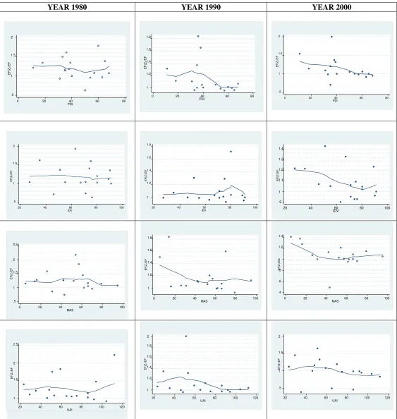
According to Daraio and Simar (2007a, b) the global influence of Z on the production process can be obtained by comparing the conditional order-m and frontier to their unconditional equivalents. In a univariate case of Z a scatter-plot of the ratios

, ( , ) / , ( , ) / , ( , ) / , ( , )

G B G B

m n m n m n m n

EF Z

x y z x y z x y x y

EF θ θ θ θ

∧ ∧ ∧ ∧

⎛ ⎞ ⎛ ⎞

= ⎜ ⎟ ⎜ ⎟

⎝ ⎠ ⎝ ⎠ (14)

against Z and its smoothed nonparametric regression line would indicate the global effect of Z on the production process. If the smoothed nonparametric regression is increasing it indicates that Z is unfavourable to environmental efficiency and when this regression is decreasing then is favourable to country’s environmental efficiency. For this purpose we use the nonparametric regression estimator introduced by Nadaraya (1964) and Watson (1964) as:

1 1 ( ) ( ) ( ) n _i i n _i i EF Z z Z K h EF g z z Z K h = ∧ = ⎛ ⎞ − ⎜ ⎟ ⎝ ⎠ =

∑

∑

3. Empirical results

The results obtained4 from the construction of , (x,y)

G n m

∧

θ , , (x,y)

B n m

∧

θ and EF

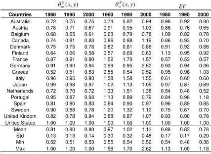
scores are presented in table 1. In most of the cases it seems that ‘bad’ efficiency increases over the years whereas ‘good’ efficiency doesn’t. This is reflected on

4

Due to the enormous quantity of results obtained it is difficult to be presented here. However all results are available upon request.

countries’ EF values. When looking the , (x,y)

G n m

∧

θ index we realize that best

performers for the three census years are reported to be: the United States, United Kindow, Japan, Portugal, France and Germany. However, when looking the

) , (

, x y

B n m

∧

θ index (i.e. producing a bad output) it appears that Australia, Canada,

France, Germany, Italy, Netherlands, Japan, Sweden and the United States appear to produce more bad output relative to the other countries. Finally, the last three columns represent the environmental efficiency indexes for those countries (see equation 10). It appears that Finland, Greece, Portugal and the United States have higher environmental efficiencies scores compare to the other countries. The interesting point regarding this finding is that those countries come from different cultural backgrounds and thus different environmental norms and values. Therefore it would be interesting to quantify the effect of those different values over the three census years over countries’ environmental efficiencies.

Table 1 about here

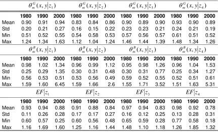
Table 2 provides descriptive statistics of the conditional measures obtained. As can be realised cultural values have a direct effect on countries environmental efficiencies’ over the years examined. For instance when looking the effect of power

distance (z1) on the G(x,yz₁)

m

θ index we realize that the average value of the standard

deviations among the efficiencies over the three census years is 0.22

[(0.2+0.21+0.27)/3]. In addition for the (x,yz1)

B m

θ

of countries’ cultural values will be also applied to countries EF performances. However it is difficult to establish that relationship looking only at the descriptive statistics provided in table 2.

Table 2 about here

Finally, figure 1 provides us with kernel density plots of the conditional environmental efficiency values. Each panel illustrates the effect of each cultural value over the three census years. The blue solid line represents the density line of the year 1980, the red dashed line for 1990 and the black dotted for 2000. It appears that the estimates conditioned to cultural values are leptokurtic for the years 1980 and 1990 in contrast with the estimates for 2000 which are appear to be in all cases platykurtic. The leptokurtic distributions indicate that there is a rapid fall-off in the density as we move away from the mean. Furthermore, the pickedness of the distribution suggests a clustering around the mean with rapid fall around it. As such it appears that cultural values in a society had influenced more countries’ environmental performance over the years 1980 and 1990 compared to year 2000. This is an indication not only of a change of the examined countries’ cultural values over the three census years but also of their effect on countries’ environmental efficiencies.

Figure 1 about here

Finally looking at the results of the year 2000 we realise that countries with higher values of power distance and individualism have a positive effect on their environmental efficiency. However countries with higher values of masculinity and uncertainty avoidance seem to have a neutral effect on their environmental efficiency. This change of cultural values through out the years is an indication of the development of environmental norms and ethics which in turn have a direct effect on countries’ environmental efficiencies. People and policy makers are now much informed regarding the problems caused to the environment from certain patterns of development and this positive effect of different cultural values on countries’ environmental efficiency is hoped to be continued over the near future.

Figure 2 about here

4. Conclusion

References

A.S.L. and Associates, 1997. Sulfur Emissions by Country and Year. Report No DE96014790, US Department of Energy, Washington DC.

An, L., Liu, J., Quyang, Z., Linderman, M., Zhou, S., Zhang, H., 2001. Simulating demographic and socioeconomic processes on household level and implications for giant panda habitats. Ecological Modeling 140, 31-49.

Bădin, L., Daraio, C., Simar, L., 2009. Optimal bandwidth selection for conditional efficiency measures: A Data-driven approach. European Journal of Operational Research doi: 10.1016/j.ejor.2009.03.038.

Berry, J.W., Annis, R.C., 1974. Ecology, culture and psychological differentiation. International Journal of Psychology 9, 173-193.

Camarero, M., Picazo-Tadeo, A.J., Tamarit, C. 2008. Is the environmental performance of industrialized countries converging? A ‘SURE’ approach to testing for convergence. Ecological Economics 66, 653-661.

Cazals, C., Florens, J.P., Simar, L., 2002. Nonparametric frontier estimation: a robust approach. Journal of Econometrics 106, 1-25.

Cherchye, L., 2001. Using data envelopment analysis to assess macroeconomic policy performance. Applied Economics 33, 407–416.

Cherchye, L., Lovell, C.A.K., Moesen, W., Van Puyenbroeck, T., 2007. One market, one number? A composite indicator assessment of EU internal market dynamics. European Economic Review 51, 749–779.

Cherchye, L., Moesen, W., Van Puyenbroeck, T., 2004. Legitimately diverse, yet comparable: on synthesising social inclusion performance in the EU. Journal of Common Market Studies 42, 919–955.

Cramer, P., Portier, K., 2001. Modeling Florida panther movements in response to human attributes of the landscape and ecological settings. Ecological Modelling 140, 51-80.

Daraio, C., Simar, L., 2006. A robust nonparametric approach to evaluate and explain the performance of mutual funds. European Journal of Operational Research 175, 516- 542.

Daraio, C., Simar, L., 2007a. Advanced robust and nonparametric methods in efficiency analysis. Springer Science, New York.

Daraio, C., Simar, L., 2005. Introducing Environmental Variables in Nonparametric Frontier Models: a Probabilistic Approach. Journal of Productivity Analysis 24, 93-121.

Daraio, C., Simar, L., 2007b. Conditional nonparametric frontier models for convex and nonconvex technologies: a unifying approach. Journal of Productivity Analysis 28, 13-32.

Deprins, D., Simar, L., Tulkens, H., 1984. Measuring labor-efficiency in post offices. In: Marchand, M., Pestieau, P., Tulkens, H., (Eds.), The Performance of public enterprises - Concepts and Measurement. North-Holland, Amsterdam, pp. 243- 267. Eriksson, R., 2005. On the ethics of environmental economics as seen from textbooks. Ecological Economics 52, 421-435.

Färe, R., Grosskopf, S., Lovell, C.A.K., Pasurka, C., 1989. Multilateral productivity comparisons when some outputs are undesirable: a nonparametric approach. Review of Economics and Statistics 71, 90–98.

Färe, R., Grosskopf, S., Tyteca, D., 1996. An activity analysis model of the environment performance of firms: application to fossil-fuel-fired electric utilities. Ecological Economics 18, 161–175.

Florens, J.P., Simar, L., 2005. Parametric Approximations of Nonparametric Frontier. Journal of Econometrics 124, 91-116.

Halkos G.Emm., Tzeremes, N.G., 2009a. Exploring the existence of Kuznets curve in countries' environmental efficiency using DEA window analysis. Ecological Economics 68, 2168-2176.

Halkos G.Emm., Tzeremes, N.G., 2009b. Measuring regional economic efficiency: the case of Greek prefectures. The Annals of Regional Science doi: 10.1007/s00168-009-0287-6.

Halkos G.Emm., Tzeremes, N.G., 2009c. Economic efficiency and growth in the EU enlargement. Journal of Policy Modeling doi:10.1016/j.jpolmod.2009.08.003.

Halkos G.Emm., Tzeremes, N.G., 2009d. Electricity Generation and Economic Efficiency: Panel Data Evidence from World and East Asian Countries. Global Economic Review 38, 251-263.

Haynes, S.K.E., Ratick, S., Bowe, S., Cummings-Saxton, J., 1993. Environmental decision models: US experience and new approach to pollution management. Environmental International 19, 261–275.

Helm, J., 1962 The ecological approach in Anthropology. American Journal of Sociology 67, 630-639.

Hofstede, G., 1980. Culture's Consequences, International Differences in Work-Related Values. Sage Publications, Beverly Hills, CA.

Liu, J., 2001. Integrating ecology with human demography, behavior, and socioeconomics: Needs and approaches. Ecological Modelling 140, 1-8.

Lovell, C.A.K., 1993. Production Frontiers and Productive Efficiency. In: Fried, H.O., Lovell, C.A.K., Schmidt, S.S. (Eds.). The Measurement of Productive Efficiency. New York, Oxford University Press.

McDonald, A., Liu, J., Prince, H., Kress, K., 2001. A socio-economic-ecological simulation model of land acquisition to expand a national wildlife refuge. Ecological Modelling 140, 99-110.

Merritt, A., 2000. Culture in the cockpit: do Hofstede’s dimensions replicate? Journal of Cross-Cultural Psychology 31, 283-301.

Mohr, E. 1994. Environmental norms, society, and economics. Ecological Economics 9, 229-239.

Nadaraya, E.A., 1964. On estimating regression. Theory of Probability Applications 9, 141-142.

Nassauer, J.I., 1995. Culture and changing landscape structure. Lanscape Ecology 10, 229-237.

Nightingale, A., 2003. Nature-society and development: social, cultural and ecological change in Nepal. Geoforum 34, 525-540.

OECD, 2008. Country statistical profiles 2008, OECD STAT Database, available from: http://stats.oecd.org/wbos/Index.aspx?usercontext=sourceoecd.

Picazo-Tadeo, A., García-Reche, A., 2007. Whatmakes environmental performance differ between firms? The case of the Spanish tile industry. Environment and Planning A 39, 2232–2247.

Redman, C.L., Grove, M.J., Kuby, L.H, 2004. Integrating Social Science into the Long-Term Ecological Research (LTER) Network: Social dimensions of ecological change and ecological dimensions of social change. Ecosystems 7, 161–171.

Shackleton, V.J., Ali, A.H., 1990. Work-related values of managers: A test of the Hofstede model. Journal of Cross-cultural Psychology 21, 109-118.

Shephard, R.W., Färe, R., 1974. The law of diminishing returns. Zeitschrift für Nationalökonomie 34, 69–90.

Silverman, B.W., 1986. Density Estimation for Statistics and Data Analysis, Chapman and Hall, London.

Simar, L., Wilson, P.W., 1998. Sensitivity analysis of efficiency scores: how to bootstrap in nonparametric frontier models. Management Science 44, 49–61.

Sondergaard, M., 1994. Hofstede’s consequences: A study of reviews, citations and replications. Organization Studies 15, 447-456.

Swierczek, F.W., 1994. Culture and conflict in joint ventures in Asia. International Journal of Project Management 12, 39-47.

Triandis, H.C., 1982. Culture’s consequences. Human Organization 41, 86-90.

Tyteca, D., 1997. Linear programming models for the measurement of environmental performance of firms: concepts and empirical results. Journal of Productivity Analysis 8, 175–189.

Weber, A., Fohrer, N., Möller, D., 2001. Long-term land use changes in a mesoscale watershed due to socio-economic factors — effects on landscape structures and functions. Ecological Modelling 140, 125-140.

Zaim, O., 2004. Measuring environmental performance of state manufacturing through changes in pollution intensities: a DEA framework. Ecological Economics 48, 37–47.

Zaim, O., Taskin, F., 2000. Environmental efficiency in carbon dioxide emissions in the OECD: A non-parametric approach. Journal of Environmental Management 58, 95–107.

Zhou P., Ang, B.W., Poh, K.L., 2008. Measuring environmental performance under different environmental DEA technologies. Energy Economics 30, 1-14.

Zhou, P., Ang, B., Poh, K., 2006. Slacks-based efficiency measures for modelling environmental performance. Ecological Economics 60, 111–118.

Zhou, P., Ang, B.W., Poh, K.L., 2007. A mathematical programming approach to constructing composite indicators. Ecological Economics 62, 291–297.

Zofio, J.L., Prieto, A.M., 2001. Environmental efficiency and regulatory standards: The case of CO2 emissions from OECD. Ecological Economics 48, 37–47.

Table 1: Descriptive statistics, unconditional environmental efficiency scores, good and bad efficiency scores

θmG(x,y) (x,y) B m

θ _EF

Countries 1980 1990 2000 1980 1990 2000 1980 1990 2000

Australia 0.72 0.75 0.75 0.74 0.82 0.94 0.98 0.92 0.80

Austria 0.78 0.71 0.67 0.91 0.95 1.03 0.86 0.76 0.65

Belgium 0.68 0.65 0.61 0.63 0.79 0.78 1.09 0.82 0.78

Canada 0.74 0.81 0.83 0.86 0.88 1.19 0.86 0.93 0.70

Denmark 0.75 0.75 0.76 0.82 0.81 0.86 0.91 0.92 0.88

Finland 0.64 0.66 0.58 0.57 0.69 0.63 1.13 0.95 0.92

France 0.87 0.91 0.90 1.52 1.70 1.57 0.57 0.53 0.57

Germany 0.91 0.90 0.94 0.99 0.95 2.62 0.93 0.94 0.36

Greece 0.52 0.51 0.53 0.55 0.54 0.52 0.95 0.96 1.03

Italy 0.96 0.95 0.93 1.58 1.58 1.55 0.61 0.60 0.60

Japan 0.99 0.98 0.97 1.02 1.13 1.09 0.97 0.87 0.89

Netherlands 0.72 0.70 0.72 1.33 1.51 1.38 0.54 0.46 0.52

Portugal 0.95 0.87 0.93 1.13 0.89 0.79 0.84 0.98 1.18

Spain 0.81 0.80 0.83 0.84 0.90 0.97 0.96 0.89 0.85

Sweden 0.90 0.88 0.78 1.20 1.32 1.12 0.75 0.67 0.70

United Kindom 0.82 0.78 0.84 0.88 0.87 1.07 0.93 0.90 0.78

United States 1.00 1.00 1.00 1.00 1.00 1.00 1.00 1.00 1.00

Mean 0.81 0.80 0.80 0.97 1.02 1.12 0.88 0.83 0.78

Std 0.13 0.13 0.14 0.30 0.32 0.48 0.17 0.17 0.20

Min 0.52 0.51 0.53 0.55 0.54 0.52 0.54 0.46 0.36

Table 2: Descriptive statistics of conditional of ‘good’, ‘bad’ and EF countries’ efficiency scores

(x,yz1)

G m

θ θmG(x,yz₂) (x,yz3)

G m

θ θmG(x,yz₄)

1980 1990 2000 1980 1990 2000 1980 1990 2000 1980 1990 2000

Mean 0.90 0.91 0.94 0.83 0.84 0.86 0.90 0.89 0.90 0.93 0.90 0.89

Std 0.20 0.21 0.27 0.16 0.15 0.22 0.23 0.23 0.21 0.24 0.21 0.19

Min 0.51 0.52 0.55 0.54 0.58 0.53 0.57 0.56 0.57 0.61 0.51 0.52

Max 1.24 1.34 1.63 1.12 1.04 1.24 1.46 1.44 1.39 1.48 1.34 1.26

(x,yz1)

B m

θ θmB(x,yz₂) (x,yz3)

B m

θ θmB(x,yz₄)

1980 1990 2000 1980 1990 2000 1980 1990 2000 1980 1990 2000

Mean 0.98 1.02 1.34 0.96 0.99 1.12 0.95 0.98 1.26 0.96 1.04 1.53

Std 0.25 0.29 1.35 0.30 0.31 0.48 0.30 0.31 0.77 0.25 0.34 1.27

Min 0.56 0.53 0.51 0.53 0.56 0.49 0.59 0.52 0.55 0.52 0.51 0.61

Max 1.59 1.60 6.45 1.59 1.66 2.6 1.55 1.71 3.52 1.51 1.63 5.31

1

z

EF EFz₂ EF z₃ EF z₄

1980 1990 2000 1980 1990 2000 1980 1990 2000 1980 1990 2000

Mean 0.93 0.94 0.88 0.91 0.88 0.84 0.97 0.94 0.83 0.98 0.92 0.78

Std 0.11 0.26 0.28 0.17 0.17 0.27 0.16 0.12 0.25 0.13 0.28 0.31

Min 0.60 0.57 0.25 0.60 0.56 0.48 0.65 0.59 0.28 0.77 0.58 0.18

Figure 2: Time representation of the Global effect of cultural dimensions on countries’ environmental efficiency

YEAR 1980 YEAR 1990 YEAR 2000

.5 1 1.5 2

20 40 60 80 100 120 UAI EF| Z1 /E F 1 1.2 1.4 1.6 1.8 2

20 40 60 80 100 120 UAI EF| Z 1 /E F 1 1.5 2 2.5

20 40 60 80 100 120 UAI EF| Z1 /E F .4 .6 .8 1 1.2 1.4

0 20 40 60 80 100 MAS EF| Z1 /E F 1 1.2 1.4 1.6 1.8

0 20 40 60 80 100 MAS EF| Z 1 /E F .5 1 1.5 2 2.5

0 20 40 60 80 100 MAS EF| Z 1 /E F .9 1 1.1 1.2 1.3 1.4

20 40 60 80 100

IDV EF| Z 1 /E F 1 1.2 1.4 1.6 1.8

20 40 60 80 100

IDV EF| Z1 /E F .5 1 1.5 2

20 40 60 80 100

IDV EF| Z1 /E F .5 1 1.5 2

0 20 40 60 80

PDI EF| Z1 /E F 1 1.2 1.4 1.6 1.8

0 20 40 60 80

PDI EF| Z1 /EF .5 1 1.5 2 EF| Z1 /EF

0 20 40 60 80