Unemployment accounts

Munich Personal RePEc Archive

Unemployment accounts

Setty, Ofer

12 April 2012

Unemployment Accounts

Ofer Setty

Tel Aviv University

April 12, 2012

Abstract

Unemployment Accounts (UA) are mandatory individual saving accounts that can be used by governments as an alternative to the Unemployment Insurance (UI) system. I study a two tier UA-UI system where the unemployed withdraw from their unemployment account until it is exhausted and then receive unemployment bene…ts. The hybrid policy provides insurance to workers more e¢ciently than a traditional UI because it provides government bene…ts selectively. Using a structural model calibrated to the US economy, I …nd that relative to a two tier UI system the hybrid policy leads to a welfare gain of 0.9%.

JEL Classi…cation: E24; E61; J64; J65

Keywords: Unemployment Accounts; Unemployment Insurance; Job-search; Moral hazard; Mechanism Design; Optimal Policy;

1

Introduction

Unemployment Accounts (UA) are mandatory individual saving accounts that can be

used by governments as an alternative to the Unemployment Insurance (UI) system.

In this paper I study the welfare implications of implementing a UA system in the

United States. The importance of such a study is re‡ected even in the pre-crisis 2007

statistics: state UI programs paid $32 billion in unemployment bene…ts to 7.6 million

un-employed workers1_{. As noted by Feldstein (2005), these policies are particularly important}

because of their impact on macroeconomic performance.

UA work as follows. During employment, the worker is mandated to save a fraction

of her labor income in an individual saving account. The worker is entitled to withdraw

payments as a fraction of her last earnings (a “replacement rate”) from this account only

during unemployment. At retirement the residual balance is transferred to the worker. A

system of UA was implemented in Chile in 2002 and it is debated whether such a system

should be implemented in the United States and in other countries, e.g., Feldstein (2005),

Orszag and Snower (2002), and Sehnbruch (2004). In contrast to this system, the UI

system is based on government bene…ts that are …nanced by a payroll tax and provided

for a limited duration.

I study a hybrid UI-UA policy that combines elements of each of the two policies.

For simplicity, I refer to the hybrid policy henceforth as UA policy. According to this

policy upon unemployment the worker is allowed to withdraw payments from her account

at a certain rate. Once the account is exhausted the worker receives unemployment

bene…ts according to a replacement rate as in a traditional UI system. This hybrid

system is conceptually di¤erent from a pure UA system in which no government bene…ts

are provided to workers2_.

1_{U.S. Department of Labor (2008). "Unemployment Insurance Data Summary," available at:}

http://www.ows.doleta.gov/unemploy/content/data.asp. Accessed on October 27, 2009.

2_{A pure UA can be considered for reasons such as myopic agents and a government who cannot}

UA deposit rate

Employment

Deposits, Withdrawals & Benefits

UA replacement rate _{UIreplacement rate}

Unemployment Time Employment Unemployment Time

Unemployment Account

Mandatory deposit

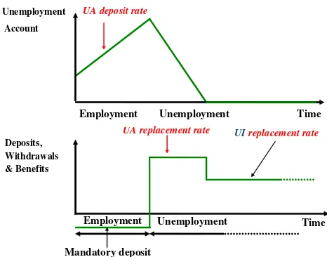
Figure 1. The UA System.

Figure 1 shows a graphic representation of the UA system for a worker who starts

o¤ employed, becomes unemployed and remains unemployed inde…nitely. The top panel

of the …gure shows the balance of the unemployment account. The balance increases

gradually during employment and then declines gradually during unemployment. Once

the balance is exhausted the account remains at its lower bound of 0.

The bottom panel of Figure 1 shows the deposits, withdrawals and transfers for that

worker. During employment the worker pays her mandated contribution to the

unemploy-ment account. Upon unemployunemploy-ment, the worker withdraws payunemploy-ments from the account

at a pre-speci…ed rate until the account is exhausted at some replacement rate. From

that point on, conditional on unemployment, the worker receives unemployment

bene-…ts according to some replacement rate, which in this example is lower than the …rst

replacement rate.

Unemployment tax Employment

Taxes & Transfers

UI replacementrate 1

UI replacementrate 2

Unemployment Time

Duration of UI benefits

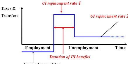
Figure 2. The UI system.

Notice that in the UA system while withdrawals from the account are based on the

worker’s own resources, unemployment bene…ts are paid from the pooled resources.

As in the UA system, I allow two tiers of payments in the UI system. Figure 2 shows

a graphic representation of the two-tier UI policy (henceforth UI) for the same worker

examined above. During employment, the worker pays an unemployment tax. Upon

unemployment, the worker receives bene…ts proportional to her last earnings, for the

duration of UI bene…ts. From the time limit of the …rst replacement rate, the worker

receives unemployment bene…ts according to the second replacement rate.

Two di¤erences between the systems should be emphasized. First, while the maximum

duration of bene…ts in UI is …xed, the duration of withdrawals in UA depends on the

balance of the unemployment account at the beginning of the unemployment spell, which

varies across workers. Second, in contrast to the UA system that uses a combination of

private and public resources, UI uses only public resources.

In order to study the welfare e¤ects of a shift from UI to UA, I build an heterogeneous

agents, incomplete-markets life-cycle model, in which workers face income ‡uctuations and

unemployment shocks. Workers in the model di¤er along several key dimensions including

age, unemployment risk, income and wealth. Unemployment in the model is driven both

by exogenous factors (layo¤s for employed workers and search frictions for unemployed

for unemployed workers). There are no aggregate shocks in this economy.

In the model the government can implement either a UI or a UA system, each

com-posed of two-tiers. The UI policy is modeled as a choice of two replacement rates, and a

time limit of the …rst replacement rate. The UA policy is modeled as a choice of a deposit

rate into the account during employment, a replacement rate funded by the mandatory

account, and a replacement rate used from the exhaustion of the mandatory account

onwards.

Given the unemployment policy, workers allocate their resources optimally between

consumption and savings. In addition, workers with employment opportunities choose

between employment and unemployment. The government takes into account these

en-dogenous decisions when designing the parameters of the unemployment system in order

to maximize the welfare of the workers. I refer to the combination of instruments that

delivers the highest welfare level in each type of system (UI or UA) as optimal UI and

optimal UA, respectively3_.

Compared with the economy under the optimal UI policy, under the optimal UA

policy the unemployment rate increases and the tax rate decreases. These two e¤ects

can happen simultaneously because the UA policy delivers bene…ts to workers selectively

and thus provides more insurance with lower resources. The e¢cient insurance leads to

a decrease in precautionary savings under the UA policy. Since workers save less under

the UA policy they can better smooth their consumption over the life cycle. This makes

workers better o¤ under the UA policy. Quantitatively, the welfare gain associated with

a shift between the two steady states, measured as a consumption equivalent variation, is

0.9%.

From a distributional perspective, the welfare gain is positive for all deciles of initial

wealth. This means that the gain associated with a shift from UI to UA is not based on

3_{Formally, these policies are sub-optimal because they are based on a limited number of instruments}

redistribution from rich to poor utilizing the di¤erences between marginal utility. Instead,

the gain is due to an increase in the insurance e¢ciency, striking a better balance between

incentives and insurance.

Yet, not all initial deciles experience the same gain, as it decreases monotonically

with assets. Poor workers are those who bene…t from the shift the most because given

their lower levels of assets they particularly bene…t from lower precautionary savings and

consumption smoothing.

To put the welfare gain of the shift from UI to UA in context, I compare the optimal

UI to two other policies within the UI policy set. The …rst is the actual UI policy in the

US, providing a …rst replacement rate of 50% for 6 months. The second is a Laissez-faire

UI policy, providing neither …rst nor second tier bene…ts.

Compared with the Laissez-faire policy, the optimal UI policy provides insurance that

increases both the tax level and the unemployment rate. This insurance leads to a welfare

gain of 0.4%. Compared with the actual UI, the optimal UI improves welfare by only

0.1%. Thus, the optimal UI can be seen as …ne tuning the instruments of the UI policy.

The welfare gains associated with a shift from optimal UI to either actual UI or

Laissez-faire are small relative to the welfare gain of a shift from optimal UI to optimal UA. This

is an important …nding because it shows that the welfare change following a shift from

UI to UA does not come from sensitivity of the welfare to the policy.

I show that the main results are robust to several forces that could theoretically a¤ect

the results. First, I show that allowing the option of deferring bene…ts in the UI policy

does not bridge over the welfare gain between the two policies. Second, I show that

changes in the role of moral hazard in the model does not a¤ect the results. Finally, I

show that the e¤ect of general equilibrium prices, had they been present in the model,

would only strengthen the main result.

Related literature

studies the design of Optimal Unemployment Insurance policies. These papers use

re-cursive contracts to formulate a parsimonious relationship between the principal (the

government) and the agent (the worker) that is based on the whole labor history of the

worker.

The seminal paper by Hopenhayn and Nicolini (1997) shows that in the optimal

con-tract, bene…ts should decline during unemployment, and the labor tax upon re-employment

should increase. These two mechanisms guarantee that it is worthwhile for the worker

to exert a high job-search e¤ort level during unemployment, because the outcome of

em-ployment is at least as good for her as the outcome of unemem-ployment4_.

The recursive contracts setting is the appropriate framework for characterizing optimal

contracts. One technical limitation of this framework, however, is the inclusion of workers’

savings in this model5_{. For the analysis of UA, allowing workers to save is crucial because}

savings determine the self-insurance level of workers in the economy. Indeed, the literature

has established that the addition of savings has important implications for the UI policy

(e.g., Shimer and Werning (2008), Kocherlakota (2004)). In addition, the importance

of long term contracts reduces signi…cantly when savings are allowed (e.g., Hansen and

Imrohoroglu (1992) and Abdulkadiroglu, Kuruscu, and Sahin (2002)).

Another important advantage of short-term contracts is that they are relatively easy

to implement. Indeed, the design of policies in this paper is closely linked to actual

unemployment systems throughout the world. Nevertheless, I am still able to adopt the

main insights of the Optimal Unemployment Insurance literature. In fact, Pavoni (2007)

shows that when there is a lower bound on the level of utility provided to the worker the

optimal UI policy resembles a two-tier UI system as the one I incorporate in this paper.

The literature on the UA policy includes several papers that compare variants of UA to

4_{Usually, this framework is used to study the unemployment insurance as the sole policy. Some}

exceptions are . Pavoni and Violante (2007) and Pavoni, Setty, and Violante (2010) who study various labor market policies targeted to the unemployed, called Welfare-to-Work programs.

5_{Abraham and Pavoni (2008) study a problem where agents have secret access to the credit market}

UI. Pallage and Zimmermann (2010) use a full blown dynamic general equilibrium model

with heterogeneity in employment and wealth to compare the two policies. Their model

is based on one saving account that includes both voluntary and mandatory savings. In

this economy few workers let their unemployment accounts deplete. They …nd that the

bene…ts upon exhaustion of the mandatory account can be signi…cantly higher that those

under a UI system. This leads to more e¢cient insurance and workers preferring the UA

system over the UI one.

Brown, Orszag, and Snower (2008) use a two period model to compare a UI system

with no savings to a UA system. Their model captures qualitatively the di¤erence in

employment incentives between the two. They show that UA changes the employment

incentives of workers and could achieve reductions in unemployment without reducing the

level of support to the unemployed.

Feldstein and Altman (2007) perform an accounting exercise based on the PSID data.

They show that a saving rate of 4% of labor income is su¢cient for …nancing the

unem-ployment bene…ts of the vast majority of workers, leading to negative balances of only 5%

of workers at retirement, death or upon exiting the panel. In addition, they show that

the cost of forgiving the negative balances (which is the only usage of the unemployment

tax) is roughly half of the cost of the unemployment insurance system.

2

The model

This section has four parts. First, I describe the economic environment of the model.

This environment is invariant to the government’s activities including the unemployment

system. Second, I introduce the government and explain in detail the unemployment

policies (UI and UA), the Social Security policy and other government expenditures.

Third, I present the worker’s optimization problems under each unemployment policy.

and maximize their utility. In the fourth and last subsection, I describe the optimal

unemployment policy for each system as the choice of the system’s instruments over the

relevant policy space that maximizes workers’ welfare.

The model is rich in especially two aspects. First, workers are heterogeneous in several

dimensions including age, unemployment risk, wealth and income. This richness is

im-portant for analyzing the welfare gain or loss of various demographic groups. Second, the

model includes a detailed productivity process, government expenditures and Social

Se-curity transfers. These details are important for matching the net resources that workers

have over the life-cycle and across labor market states.

2.1

The economy

2.1.1 Demographics

The model is in discrete time. The economy is stationary, i.e., there are no aggregate

shocks. Workers are born at date 1, and live up to T periods. Throughout the life-cycle

workers face an age-dependent unconditional survival rate t:

The life-cycle [1; T] is split into two periods. During age [1; TR 1] workers are in

the labor force and can be either employed or unemployed. I abstract from labor-force

entry and exit considerations since unemployment payments are conditional on being

attached to the labor force. During age [TR; T] workers are retired. I refer to the time

span[1; TR 1]as theworking age,and to the time span of [TR; T]as theretirement age.

2.1.2 Preferences

Workers’ period utility is u(c) Bq where c is consumption, B is disutility from work

and q is an employment indicator that equals 1 if the worker is employed and 0 if the

maximize:

U =E₀

( _T X

t=1

t t 1[u(ct) Bqt]

)

where:

qt =

(

1 if employed at time t

0 otherwise

2.1.3 Labor market and timing

Job Offer

) (πt

No Job Offer

) 1 ( −πt

Accept/ Reject

Accept Reject Unemployed

Unemployed

Employed Unemployed Not Laid Off

) 1 ( −ψt

Laid Off

) (ψt

Retain/ Quit

Retain Quit Unemployed Employed

Employed Unemployed

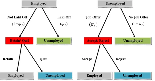
Figure 3. The Labor Market and the Timing of the Model.

Figure 3 shows the labor market structure and the timing of the model for employed

and unemployed workers6_{. An employed worker is laid o¤ and becomes unemployed with}

probability _t that depends on her age t. A worker that is not laid o¤ decides whether

to retain or to quit the job. If the worker retains her job, then she remains employed.

The process for an unemployed worker is similar. An unemployed worker with an

unemployment duration of d receives at the beginning of the period a job o¤er with age

dependent probability t. If the worker does not receive a job o¤er then she remains

unemployed. A worker that receives a job o¤er decides whether to accept the job o¤er

6_{The model does not include a choice of intensive margin mainly because UI in most states in the US}

and become employed or reject it and remain unemployed. I discuss the observability of

quits and job-o¤er rejections later on, when I introduce the government.

The design of the transitions between employment and unemployment therefore allows

both exogenous factors and endogenous decisions. The presence of endogenous decisions

is a key component in the model as it implies that unemployment is determined within

the model and depends on the unemployment policy7_.

2.1.4 Labor productivity process

Workers face a standard individual labor productivity process that accounts for a life-cycle

trend and persistent income shocks. The log labor income of an employed individuali at

aget is:

yi;t = kt+zi;t

zi;t = zi;t 1+ i;t

The …rst component, kt, is a life-cycle trend that accounts for the return to experience

over the life-cycle and supports the hump shape of labor income towards retirement.

The second component, zi;t; is an AR(1) process with persistence , and innovations

i;t N

2

2 ;

2 _{: The initial persistent shock is distributed z}

i;1 N

2 1

2 ; 2

1 , thus

allowing for initial heterogeneity in earnings already at date 1.

During unemployment, the persistent component of labor income is constant. This

formulation is useful for recovering the last labor income, which is the basis for

unem-ployment payments in both systems.

7_{An alternative model of the labor market would include a search e¤ort that a¤ects the job …nding}

2.1.5 Initial wealth and savings

Workers are born at date 1 with an initial wealth of ai;1. The log of initial wealth is

distributedN 2a

2 ; 2

a :Workers can save and borrow up toa, and the periodic interest

rate on assets is r:

2.2

The government

The government implements an unemployment policy (either UI or UA) for insuring

work-ers against unemployment, a Social Security system for retired workwork-ers, and a government

expenditure.

2.2.1 The UI system

The UI policy includes three instruments (see Figure 2). The …rst instrument is the

dura-tion of the …rst tier bene…ts, denoted by DU I: The second instrument is the replacement

rate, Q1

U I, used up to the time limit DU I. This instrument determines for each worker

the level of bene…ts during the …rst tier of unemployment. The third instrument is the

replacement rate once the duration of the …rst tier bene…ts is completed, denoted byQ2_{U I}:

The second tier bene…ts do not have a time limit. All bene…ts are taxable.

Following the UI policy in the US, UI bene…ts are only provided to workers who were

laid o¤. Workers who quit are ineligible to bene…ts. The implied assumption of this

restriction is that quits are observed by the government. This assumption is supported by

a component of the UI system called "experience ratings", that indexes the unemployment

tax rate to the layo¤s experience of the …rm. Thus, a …rm that reports a quit as a layo¤

would, in general, face a higher unemployment tax rate. This guarantees that the …rm

has the incentive to report the truth. For more on experience ratings see Wang and

Williamson (2002).

Rejections of job o¤ers, on the other hand, are assumed to be unobservable by the

involve a third party that has no interest in reporting the job-o¤er rejection. Although

some monitoring of such rejections takes place in the US, Setty (2012) shows that the

average monthly monitoring probability in the US is 0.20. This is an upper bound for the

probability of observing a rejection because some rejections are undetected. I therefore

assume that job-o¤er rejections are perfectly unobservable.

2.2.2 The UA system

The UA policy includes three instruments (see Figure 1). The …rst instrument is the

mandatory saving rate during employment, denoted byMU A:This instrument, which is a

fraction of labor earnings, determines thein‡ow into the account. The second instrument

is the replacement rate, denoted by Q1_{U A}, provided by withdrawals from the account.

This instrument determines the out‡ow from the account. The third instrument is the

replacement rate once the mandatory account is exhausted, denoted byQ2_{U A}:As in the UI

system, these second tier bene…ts do not have a time limit. Upon retirement, the balance

of the mandatory account becomes available for the worker.

I assume that the mandatory account bears the same periodic interest, r, as private

saving8_{. Note that given that the return on the two assets is the same and that the}

liquidity of the mandatory account is lower, the worker would always prefer to deposit

the minimum amount in the account, and withdraw the maximum amount from the

account.

The mandatory account has an upper bound am and a lower bound of 0: The upper

bound is used for technical convenience only and will be calibrated to a level that has no

e¤ect on welfare compared with a choice of no bound9_{. Relaxing the assumption that the}

8_{The return on the mandatory savings could be di¤erent than that of the regular savings for at least}

three reasons: higher regulation on the investment (to avoid moral hazard among other reasons); a higher interest rate given the central management of the funds; and an overhead cost. I abstract from these considerations and leave them to further research.

9_{Retirement is an important reason for saving in the model. Since the mandatory account becomes}

lower bound of the mandatory account is0and allowing workers to have negative balances

would generate another instrument - allowing workers to borrow against their future

income. This idea was suggested by Stiglitz and Yun (2005) and can be implemented in

the current framework as well.

I assume for consistency with the UI system that only laid o¤ workers are eligible for

withdrawing from the unemployment account and for second tier bene…ts10_.

The UA system described here is inspired by the UA system implemented in Chile

with the key di¤erence of the additional UI tier as opposed to a minimal transfer in the

Chilean system. Appendix A presents the Chilean system in detail and describes these

di¤erences.

2.2.3 Other government activities

In addition to the unemployment policy, the government administers two other activities.

The inclusion of these activities is important for setting the conditions that workers face

during employment and retirement.

The …rst activity is retirement payments to retired workers. This activity follows the

two main principles of the Social Security retirement plan in the US. Speci…cally, payments

are based on lifetime earnings and payments are progressive. The retirement policy in

the model di¤ers from the actual retirement policy in the US in the way lifetime savings

are calculated. Since lifetime earnings in the model are not part of the worker’s state,

they are approximated by the worker’s last observed labor income. This approximation

is explained in the calibration section.

The second activity is government expenditure, denotedG. The government spends a

…xed amount on exogenous expenditures that do not bene…t workers. These expenditures

high enough as to not make continually employed workers eligible for second tier bene…ts.

10_{Since the worker is using her own resources to …nance the unemployment bene…ts, it would be}

are important for setting the correct average labor tax distortion that workers face.

The government …nances its three activities (the unemployment system, Social

Se-curity, and government expenditure) by collecting a labor income tax for either UI or

UA, denoted by U I _and U A_{, respectively. Note that these two alternative taxes are not}

decision variables, but rather used to balance the government budget.

2.2.4 Information structure

Mandatory savings are regulated by the government and hence are observable by both

the government and the workers. Private individual savings are unobservable to the

government.

2.3

The worker’s problems

2.3.1 UI

The worker’s state under the UI system is composed of …ve components: age (t);private

savings (a);persistent component of labor income (z); unemployment duration (d), and

eligibility for unemployment bene…ts(e):

Workers in the model have two types of decisions. The …rst type of decision is an

intertemporal decision of consumption and savings. This decision is based on a speci…c

employment state (employed or unemployed). The second type of decision is the

in-tratemporal decision of employment. This decision is relevant only for workers with an

employment opportunity (employed workers who are not laid o¤ and unemployed workers

with a job o¤er).

The values for the workers when employed and unemployed are WU I_{(t; a; z) and}

VU I_{(t; a; z; d; e) respectively. These values are the outcome of an intertemporal}

maxi-mization over consumption and savings. Note that the value for the employed worker

does not include unemployment duration and eligibility, which are only relevant for the

The values for workers with job opportunities are given as follows. The value for a

worker who was employed in the previous period and was not laid o¤ is JU I

w (t; a; z).

The value for a worker who wasunemployedin the previous period and has a job o¤er

is JU I

u (t; a; z; d; e). These values are the outcome of an intratemporal maximization over

a choice between employment and unemployment:

J_uU I(t; a; z; d; e) = max

faccept;rejectg W

U I

(t; a; z); VU I(t; a; z; d; e) (1)

J_wU I(t; a; z) = max

fretain;quitg W

U I

(t; a; z); VU I(t; a; z;1;0) (2)

The value for an unemployed worker who holds a job o¤er, JU I

u ( ); is determined

as a choice between becoming employed (accept) and remaining unemployed (reject).

Note that since rejections are unobservable by the government the eligibility of remaining

unemployed (e) is carried unchanged to unemployment.

Similarly, the value for an employed worker who does not face a layo¤ shock,JU I w ( );

is determined as a choice between remaining employed (retain) and becoming unemployed

(quit). Note that since quits are observable by the government the eligibility upon

be-coming unemployed(e) is 0.

Using these values, we can now de…ne the value for the employed and the unemployed

UI is:

VU I(t; a; z; d; e) = (3)

max

c;a0 u(c) + tEt tJ

U I

u (t+ 1; a0; z; d+ 1; e) + (1 t)VU I(t+ 1; a0; z; d+ 1; e)

s:t:

a0 = a(1 +r) c+x

a0 1 a

x = 8 > > > > < > > > > :

Q1_{U I}exp (kt+z) 1 U I if e= 1 and d DU I

Q2_{U I}exp (kt+z) 1 U I if e= 1 and d > DU I

0 if e= 0

9 > > > > = > > > > ;

The worker in this problem decides on current consumption (c) and future assets (a0) in order to maximize current utility from consumption and the future value. The discounted

future value is multiplied by the age-dependent conditional survival rate t: The future

value itself is a composition of the values of receiving and not receiving a job o¤er with

the respective probabilities of t and (1 t).

The …rst constraint is a standard budget constraint wherexis the government transfer.

A worker who is eligible for unemployment bene…ts and whose unemployment duration

is within the time limit of UI bene…ts, receives the …rst replacement rate of the previous

labor earnings. An eligible worker with d > DU I receives the second replacement rate.

The value for an employed worker under UI is:

WU I(t; a; z) = (4)

max

c;a0 u(c) B+ tEt (1 t)J

U I

w (t+ 1; a0; z0) + tV U I

(t+ 1; a0; z0;1;1)

s:t:

a0 = a(1 +r) c+ exp (kt+z) 1 U I

a0 1 a

Note that the eligibility state upon being laid o¤ is equal to1. Also note that the value

for the worker includes the disutility from work( B):

2.3.2 UA

The structure of the value functions for the worker under the UA policy is similar to that

of the UI. The worker’s state under the UA system is composed of …ve components as

well: age(t);private savings(a);mandatory savings(am), persistent component of labor

income(z), and eligibility for withdrawals(e):It di¤ers from the worker’s state under UI,

because of the additional mandatory savings(am), and the absence of the unemployment

duration(d):

These two changes in the state space of the worker re‡ect the criterion for

unemploy-ment payunemploy-ments: in UI it is the unemployunemploy-ment duration and in UA it is the endogenous

balance of the mandatory account.

The intratemporal value functions under UA are:

J_uU A(t; a; am; z; e) = max

faccept;rejectg W

U A

(t; a; am; z); VU A(t; a; am; z; e)

J_wU A(t; a; am; z) = max

fretain;quitg W

U A_{(t; a; a}

m; z); VU A(t; a; am; z;0)

withdrawal from the mandatory account, andb is the government transfer.

VU A(t; a; am; z; e) = (5)

max

c;a u(c) + tEt tJ U A

u (t+ 1; a0; a0m; z; e) + (1 t)VU A(t+ 1; a0; a0m; z; e)

s:t:

a0 = a(1 +r) +m+b c

a0_m = am(1 +r) m

b = 8 > > > > < > > > > :

Q2_{U A}exp (kt+z) 1 U A m if am < Q1U Aexp (kt+z) 1 U A

and e= 1

0 otherwise 9 > > > > = > > > > ; m = 8 > < > :

min Q1

U Aexp (kt+z) 1 U A ; am(1 +r) if e= 1

0 otherwise 9 > = > ;

a0 1 a

The objective function that determines VU A_{( ) is similar to the one in the value for}

an unemployed worker under UI with the necessary adjustments. Future private savings

in the …rst constraint are determined by the sum of current private savings including

the interest rate, the withdrawal from the account, and the second tier bene…ts minus

consumption.

The withdrawal for an eligible worker(m)is equal to the replacement rate of previous

earnings if the account has a su¢cient balance. Otherwise, it is the balance of the account.

The second tier bene…ts (b) are based on the second replacement rate and are provided

to workers who exhausted their mandatory account. Workers with account balances that

are lower than the second tier bene…ts receive the di¤erence in bene…ts. The mandatory

The value for an employed worker under UA is:

WU A(t; a; am; z) =

max

c;a0 u(c) B+ tEt (1 t)J

U A

w (t+ 1; a0; a0m; z0) + tV U A

(t+ 1; a0; a0_m; z0;1)

s:t: :

a0 = a(1 +r) + exp (kt+z) 1 U A c (a0m am(1 +r))

a0_m = min am; am(1 +r) + exp (kt+z) 1 U A MU A

a0 1 a

The budget constraint of the worker in the …rst constraint of WU A_{( ) includes the}

deposit to the mandatory account(a0

m am(1 +r)):This deposit is equal to the deposit

rate, times the net labor earnings as long as the account’s balance is lower than am:

Otherwise, it is the deposit that sets the mandatory account’s balance at its upper bound.

Note that the labor income used for replenishing the mandatory account is taxed, same

as with the voluntary account.

2.4

Optimal unemployment policies

The objective of each of the optimal unemployment policies is to maximize the welfare

of the workers in the economy. The welfare metric that I use is constant consumption

equivalent, de…ned as the constant consumption cthat solves:

X

E0

( _T X

t=1

t t 1[u(c) Bqt]

)

=XE0

( _T X

t=1

t t 1[u(cet) Bqet]

)

where _fc_et;qetg are the optimal consumption and employment levels under the studied

policy, and qt is the average age dependent unemployment rate under the actual UI.

When comparing two policies _fi; j_g, the welfare gain (or loss) of shifting from policyi to

policyj is measured as the consumption equivalent variation, de…ned as: ! = ci cj

fci; cjgare the constant equivalent consumption levels of policiesfi; jg, respectively. This

is the percentage increase in consumption that needs to be given to the average worker

at each date in her lifetime in the baseline policy (e.g. actual UI) to make her exactly as

well o¤ as under the suggested policy (e.g. optimal UI).

The average welfare at time 0 is weighted over the distribution of initial assets and

persistent shocks at time0with measures_{f 0};1 _0gfor time0employed and unemployed

workers.

An optimalUnemployment Insurance policy is a triplet_fD_{U I} ; Q1_{U I} ; Q2_{U I g}such that:

E0 0WU I(t= 0; a; z) + (1 0)VU I(t = 0; a; z; d= 1; e= 1) is maximized,

where the expectation operator is taken with respect to initial wealth and the initial

persistent component of income.

the government budget is balanced:

R

t<TR A Z d=0 Eexp (kt+z)

U I ₌R

t<TR A Z 1 d DU I e=1Q

1

U Iexp (kt+z) 1 U I

+R_t<T

R A Z d>DU I e=1Q

2

U Iexp (kt+z) 1 U I +

R

t TR A Z D Eexp (kt+z)g(z)+

G;

where g(z)is the determination of Social Security bene…ts based on the persistent

component of labor income.

An optimalUnemployment Accounts policy is a triplet_fM_{U A} ; Q1_{U A} ; Q2_{U A g}such that:

E0 0WU A(t = 0; a; am = 0; z) + (1 0)VU A(t= 0; a; am = 0; z; e= 1) is

maxi-mized,

the government budget is balanced:

R

t<TR A AM Z Eexp (kt+z)

U A ₌

R

(t<TR A AM Z E)b 1

U A ₊R

t TR A AM Z Eexp (kt+z)g(z) +G;

3

Calibration

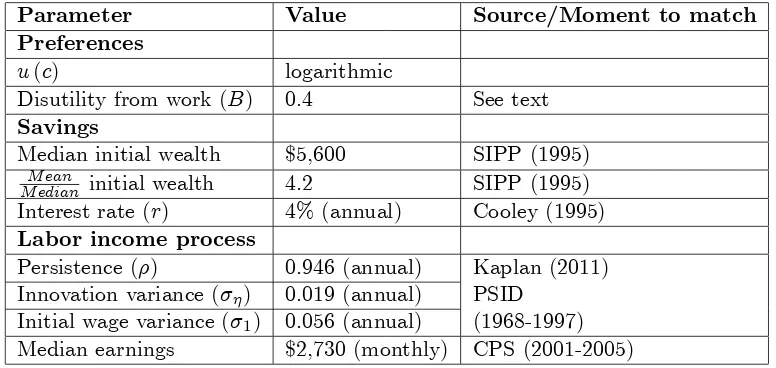
Table 1 - Externally calibrated parameters

Parameter Value Source/Moment to match

Preferences

u(c) logarithmic

Disutility from work(B) 0.4 See text

Savings

Median initial wealth $5,600 SIPP (1995)

M ean

M edian initial wealth 4.2 SIPP (1995)

Interest rate (r) 4% (annual) Cooley (1995)

Labor income process

Persistence( ) 0.946 (annual) Kaplan (2011) Innovation variance( ) 0.019 (annual) PSID

Initial wage variance( 1) 0.056 (annual) (1968-1997) Median earnings $2,730 (monthly) CPS (2001-2005)

The model is calibrated to match key moments in the US economy given the actual

UI policy in the steady state US economy.

The calibration strategy is composed of two parts. I …rst cover the parameters that are

calibrated externally to the model. These parameters are expected to a¤ect both policies

in a similar way and are used here to …ne tune the economic environment that workers

face. I then cover the parameters that a¤ect the consumption-saving and employment

de-cisions of the workers in the economy. These include the discount rate, the social security

payments, the tax rate, and the age dependent job o¤ers and separations probabilities.

Because of the importance of each of those four parameters I calibrate each of them to

match a speci…c data target.

3.1

Externally calibrated parameters

3.1.1 Life-cycle

The unit of time is one month. This frequency, which is relatively high for a life-cycle

model, supports a careful distribution of unemployment shocks. The survival rates are

taken from the US Census (2005).

Workers join the labor force at age 25 and are part of the labor force until they are

65. The retirement age of 65 is set to an age that is between the full retirement age range

in the US of 65 to 67 (depending on the year of birth) and the early retirement option at

age 62. The maximum age,T, is calibrated to 100 years of age11_.

The life-cycle therefore consists of a working age span of 40 years (or 480 months) and

a retirement age span of 35 years (or 420 months).

3.1.2 Preferences

Utility from consumption is logarithmic. The level of disutility from work,B, determines

the optimal generosity of the unemployment policy. The values for this parameter in the

literature vary between 0:25 in Ljungqvist and Sargent (2008) and 0:67 in Pavoni and

Violante (2007). For the model presented here a level of B = 0:2 would imply a very

low level of moral hazard, while a level of B = 0:6would imply a very high sensitivity of

the unemployment rate to the unemployment policy. In order to allow for the economic

forces of both policies to be active I choose an intermediate level of B = 0:4. I show in

the results section that the main results are robust to B _{2 f}0:3;0:5_g:

3.1.3 Labor productivity

The age pro…le (kt) is estimated using mean earnings with cohort e¤ects from the PSID.

See Huggett, Ventura, and Yaron (2006) for more details. The income process is based

on Kaplan (2011), where = 0:946, 2 _{= 0:019 (both annual), and the initial variance of}

the persistent shock is 2z1 = 0:056. Median monthly earnings are equal to$2;730, based

on the 2009 CPS data.

3.1.4 Savings

The initial wealth distribution is set in order to match two key moments of the assets

distribution of workers in the age bin of 25-34 years in the SIPP data (Anderson (1999)).

The …rst moment is the median net worth of $5,600. The second is the mean-median

ratio of 4.2. This asset distribution implies a high Gini of wealth of 0.78 at age 25. The

borrowing limit is set to0. The annual interest rate is set to 4% following Cooley (1995).

3.1.5 Actual UI policy in the US

The actual UI policy in the US varies across states. Nevertheless both the instruments

and their levels are fairly consistent. On average, UI bene…ts in the US are based on a

replacement rate of 50% for a duration of 26 weeks (DOL, 2011).

3.2

Parameters that are matched to speci…c moments

Table 2 summarizes the values for the parameters that are matched to speci…c moments

in the model.

3.2.1 The discount rate

The interest rate r, and the discount rate , are the key parameters that determine the

wealth-income ratio through the determination of the average savings in the economy.

The wealth-income ratio target of 2.5 is approximately the average wealth to average

income ratio computed from the 1989 and 1992 Survey of Consumers Finances (SCF),

when wealth is de…ned as total net worth, income is pre-tax labor earnings plus capital

income, and when the top 5% of households in the wealth distribution are excluded12_{. See}

12_{Note that given that the top 5% hold 54% of the net worth of wealth (Cagetti and Nardi (2006)),}

Kaplan and Violante (2010) for more details. To match this target I set the annual interest

rate to 4% (Cooley (1995)) and adjust the discount rate accordingly. The resulting value

for the monthly discount rate is 0.9973.

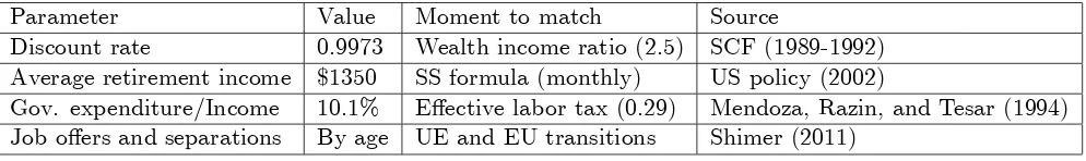
Table 2 - Parameters that are matched to speci…c moments

Parameter Value Moment to match Source

Discount rate 0.9973 Wealth income ratio (2.5) SCF (1989-1992) Average retirement income $1350 SS formula (monthly) US policy (2002)

Gov. expenditure/Income 10.1% E¤ective labor tax (0.29) Mendoza, Razin, and Tesar (1994) Job o¤ers and separations By age UE and EU transitions Shimer (2011)

3.2.2 Social Security payments

As in the US, Social Security payments for retired workers are based on the worker’s

lifetime labor earnings, which are not a part of the worker’s state. To approximate the

retirement payment for each worker, I simulate earnings paths based on the productivity

process, and regress the lifetime earnings on the last observed level of earnings. The

resulting formula is used to approximate lifetime earnings on the last observed earnings

in the model. The approximation is fairly good. The variation of the last earnings level

explains 85% of the variation in lifetime earnings. This is due to the high persistence in

the productivity process.

3.2.3 Government expenditure

The Government expenditure is set to match the e¤ective tax rate of 0.29 of Mendoza,

Razin, and Tesar (1994) for 1995-1998. This tax is split between the transfers of UI (2.3

percentage point), Social Security (17.3 percentage point), and government expenditure

(10.1 percentage point). The equivalent amount of government expenditures remains

…xed throughout the experiments of both UI and UA. Therefore the government

Figure 4. Model First Moments.

3.2.4 Unemployment in‡ows and out‡ows

The initial employment level is set according to the unemployment rate at age 25. The

target age-dependent transitions between employment and unemployment are taken from

Shimer (2011). These values are based on the period of 1990-2005 from the CPS data.

Since these are a¤ected by both exogenous factors (separations and the absence of job

o¤ers) and endogenous decisions (quits and rejections of job o¤ers) I factor the data

transitions and use these as the exogenous driving forces for unemployment ( t and t).

I choose this factor such that the average unemployment in the model equals the average

Figure 5. Model Second Moments.

3.3

Model moments

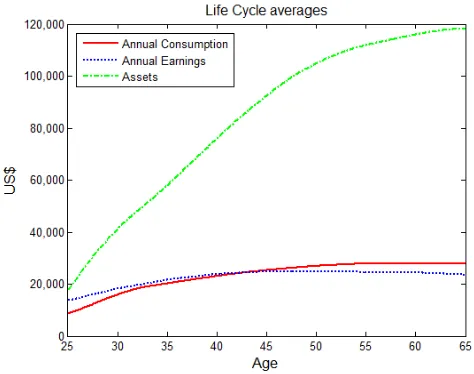
Figure 4 shows the life cycle means of annual consumption, annual net earnings and assets

in the simulation for the actual UI policy. The …gure shows that the model has reasonable

implications for these variables over the working age. Assets increase over the life cycle,

and ‡attens at age 55. The savings at age 65 is used by workers as a bu¤er for retirement,

given the low replacement rate of Social Security. Consumption in the …rst part of life

is lower than earnings. This is because workers save for precautionary reasons to insure

themselves against unemployment shocks and negative income shocks. In the second part

of life, consumption is higher than earnings as precautionary savings are less needed.

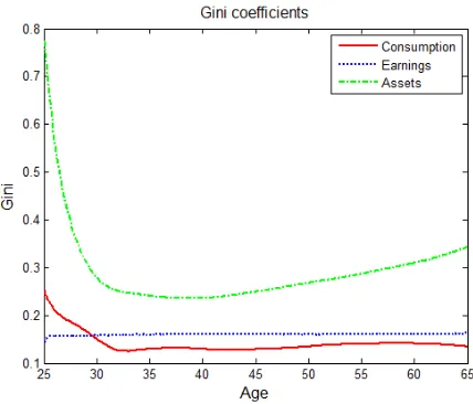
Figure 5 shows the Gini coe¢cients of consumption, earnings and assets. The Gini

coe¢cient of assets starts at a high level that is matched to the data and decreases

dramatically as workers with low assets save for precautionary reasons. Then it increases

Figure 6. The Employment Level in the Data and in the Model.

The Gini coe¢cient of consumption is relatively high at the beginning of life because

poor workers who face either unemployment shocks or negative income shocks have too

little assets for smoothing their consumption. The Gini coe¢cient of earnings increases

slightly over the working age. This is due to the already existing variance of the persistent

shock at age 25.

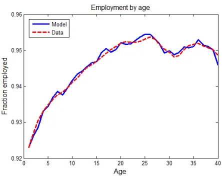
Figure 6 compares the data and model employment rate over the working age. The …t

is a result of allowing both in‡ows and out‡ows of unemployment to be age-dependent.

The fact that the two employment pro…les are similar across all ages implies that the

endogenous employment decisions are somewhat uniform across all age groups.

4

Results

In this section I report the cross section statistics of the economies under the optimal UI

and the optimal UA policies and the resulting welfare gain. I then compare the optimal UI

to the actual UI and to a Laissez-faire policy in order to put the welfare gain in context.

I conclude this section with a robustness analysis.

the three instruments of each policy, resulting in 567 combinations for UI or UA. The

computational method is described in details in Appendix B.

4.1

Optimal UI versus optimal UA

Table 3 presents the instruments and the cross-section statistics for the optimal UI and

the optimal UA policies along with the welfare gain for a shift from the optimal UI to the

optimal UA policy.

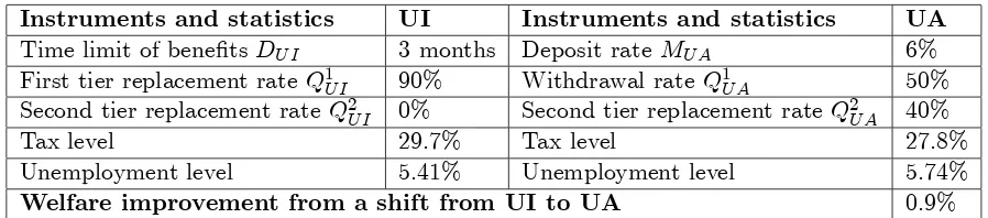
Table 3 - Optimal UI versus Optimal UA

Instruments and statistics UI Instruments and statistics UA

Time limit of bene…tsDU I 3 months Deposit rateMU A 6%

First tier replacement rateQ1_{U I} 90% Withdrawal rateQ1_{U A} 50% Second tier replacement rateQ2_{U I} 0% Second tier replacement rate Q2_{U A} 40%

Tax level 29.7% Tax level 27.8%

Unemployment level 5.41% Unemployment level 5.74%

Welfare improvement from a shift from UI to UA 0.9%

The optimal UI policy provides a high replacement rate of 90% for a duration of

3 months13_{. The second tier bene…t for the optimal UI is 0%. The choice of the two}

replacement rates in this policy takes into account that by construction all unemployed

workers are entitled to those types of bene…ts. Compared with the actual UI, this policy

leads to an increase in the tax rate of 0.7% and keeps the unemployment rate unchanged.

The optimal UA policy is based on a saving rate of 6% and a withdrawal rate of 50%.

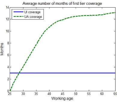
Figure 7 shows the average months of the coverage of the …rst tier bene…ts in UI and

withdrawals in UA over the life cycle. The UI coverage is the duration of the optimal UI

of 3 months. The UA coverage is equal to the average mandatory assets divided by the

withdrawal level. While the UI coverage is age neutral, the UA coverage increases rapidly

over the life cycle. This is a result of the ratio between withdrawals and savings relative

to the unemployment rate.

13_{The high replacement rate is possible since the transition from employment to unemployment is not}

The duration of the withdrawals under the UA policy is a key variable of the optimal

UA policy. The withdrawal rate is …nanced by the workers mandatory account and it

delays the government bene…ts. This allows the second tier bene…ts to be relatively high,

standing at 40%, compared with 0% under the optimal UI policy. This is especially

signif-icant since second tier bene…ts are provided without a time limit. This high replacement

rate can be provided for a long duration since it is only granted to a minority of the

unemployed workers.

Fig. 7. The Average Number of Months of First Tier Ccoverage for UI and for UA.

Compared with the UI economy, in the UA economy the unemployment rate increases

and the tax rate decreases. These two e¤ects can happen simultaneously because the UA

policy delivers bene…ts to workers selectively and thus provides more insurance with lower

resources. Compared with an unemployment tax of 2.3 percentage points (out of 29.7%)

in the optimal UI, the unemployment tax in the optimal UA policy, which is the tax

required to …nance the second tier bene…ts is only 0.3 percentage points (out of 27.8%).

These 0.3 percentage points are provided exactly to those unemployed workers who need

it the most.

In order to understand the e¤ect of the e¢cient insurance on workers’ welfare we

need to analyze the response of workers to the two optimal policies by looking at the

Figure 8 shows the average assets over the life cycle under the optimal UI and UA

policies. The savings for UI are the voluntary savings, whereas for UA it is the sum of

voluntary and mandatory savings. The UA assets diverge downwards until around age

40. At age 50 most of the labor market risk is over and UA assets converge towards the

UI assets.

The e¢cient insurance in UA allows workers to decrease their precautionary savings

for unemployment shocks. This is the case since the second tier bene…ts in UA provide

good insurance against long unemployment spells that require high precautionary savings.

Note that other motives for savings such as retirement and income ‡uctuations are kept

constant between the two economies14_.

Since young workers save less under the UA policy they can better smooth their

consumption over the life cycle. This can be seen in Figure 9 that shows the life cycle

average monthly consumption under the two systems15_{. Quantitatively, the welfare gain}

associated with a shift between the two steady states is 0.9%.

Figure 8. UI and UA Average Life Cycle Savings.

14_{The mandatory savings under the UA have a strong substitution with the voluntary savings for}

retirement, as both types of savings can be used equivalently to …nance consumption during retirement.

15_{The importance of consumption smoothing over time is also emphasized in Michelacci and Ru¤o}

Figure 9. UI and UA Average Life Cycle Consumption.

4.1.1 Distributional welfare change

The existence of heterogeneity in the model across age, employment risk, wealth and

income, implies that the average welfare change already accounts for di¤erent types of

workers in the economy. Nevertheless, it is of interest to look at the welfare change of the

shift from UI to UA across initial wealth, which is a key source of heterogeneity in the

model.

Figure 10 shows the welfare gain over the ten deciles of initial assets. Observe that

the welfare gain is positive for all deciles of initial wealth. This means that the gain

associated with a shift from UI to UA is not based on redistribution from rich to poor

utilizing the di¤erences between marginal utility. Instead the gain is due to an increase

in the insurance e¢ciency, striking a better balance between incentives and insurance.

As expected, the welfare gain decreases monotonically with assets. Poor workers are

those who bene…t from the shift the most because given their lower levels of assets they

particularly bene…t from lower savings and consumption smoothing. Workers in the top

decile of initial assets are much less concerned about the unemployment policy because

most of their consumption is based on their assets rather than on their labor income.

4.2

Optimal UI in context

To put the welfare gain of the shift from UI to UA in context, it is useful to compare

the optimal UI to two other policies within the UI policy set. The …rst is the actual UI

policy in the US, providing a …rst replacement rate of 50% for 6 months. The second is a

Laissez-faire UI policy, providing neither …rst nor second tier bene…ts. Table 5 shows the

instruments’ values and the cross-sectional statistics for these two policies along with the

optimal UI. The welfare gain is calculated in this table with respect to the Laissez-faire

policy.

Table 4 - Laissez-faire versus Optimal UI and Actual UI Policies

Instruments and statistics Laissez-faire Optimal UI Actual UI Time limit of bene…tsDU I (months) 0 3 6

First tier replacement rateQ1_{U I} 0% 90% 50% Second tier replacement rateQ2_{U I} 0% 0% 0%

Tax level 27.3% 29.7% 29.0%

Unemployment level 5.37% 5.41% 5.41%

Welfare gain relative to Laissez-faire 0.4% 0.3%

The Laissez-faire UI policy provides no unemployment bene…ts (Q1_{U I} = Q2_{U I} = 0).

and social security) are exactly the same as before, allowing an analysis of the speci…c

e¤ect of the UI bene…ts. As expected, this policy increases employment and decreases the

tax rate in the economy.

Compared with the Laissez-faire policy, the optimal UI policy provides insurance that

increases both the tax level and the unemployment rate. This insurance leads to a welfare

gain of 0.4%. Here, too, the welfare gain is especially high for poor workers, standing at

1.1% for workers in the lowest decile of initial assets.

Compared with the actual UI, the optimal UI improves welfare by only 0.1%. Thus,

the optimal UI can be seen as …ne tuning the instruments of the UI policy. Compared

with the welfare gain of a shift from optimal UI to optimal UA of 0.9%, the welfare gains

associated with a shift from optimal UI to either actual UI or Laissez-faire are small. This

is an important …nding because it shows that the welfare change following a shift from

UI to UA does not come from sensitivity of the welfare to the policy.

Interestingly, a policy that is remarkably close to the actual UI policy gets very near

to the optimal UI policy, inferior by less than 0.05%. This near-optimal policy provides

a …rst tier replacement rate of 50% for 6 months, exactly as the actual UI policy, but it

is followed by a second replacement rate of 10%.

Although the optimal and the near-optimal policies score almost the same welfare

level the distributional welfare is quite di¤erent. Figure 11 shows the welfare gain and

loss for a shift from the optimal UI to the near optimal UI. Compared with the optimal

UI, the near optimal policy UI increases the welfare of initial assets deciles 1-4, keeps

the 5th decile indi¤erent, and reduces the welfare of the rest of the deciles. This welfare

distribution demonstrates the tension between incentives and insurance in the model and

the sensitivity of poor workers to the level of insurance16_.

16_{The …rst replacement rate of the near optimal UI is consistent with the one that Chetty (2008)}

Figure 11. Optimal UI to Near Optimal UI Welfare Gain and Loss by Initial Assets.

4.3

Robustness

In this section I examine several forces that could a¤ect the results. I consider the following

three cases. First, I show that allowing the option of deferring bene…ts in the UI policy

does not bridge over the welfare gain between the two policies. Second, I study the

response of the optimal policies to the level of moral hazard in the model by changing

the parameter of disutility from work. Third, I discuss the expected general equilibrium

e¤ects on the results.

4.3.1 Deferred UI

The better insurance that is provided in UA is driven by the information carried in the

mandatory account. This information allows the government bene…ts to be conditional

on past labor history. In contrast, under the UI policy workers receive bene…ts as soon

as they become unemployed. To demonstrate the importance of selectively deferring

bene…ts in UI, I allow the UI policy to include one more instrument - the number of

months of delaying bene…ts. Under this new policy workers self insure themselves during

The optimal policy under that extended instruments UI policy is a delay of one month

in the bene…ts followed by 0.7 replacement rate for 3 months and a zero second tier

ben-e…ts. Compared with the previous UI optimal policy (where bene…ts cannot be deferred)

the welfare gain is 0.1%. This modest increase demonstrates the importance of deferring

the bene…ts only to workers with good labor market histories.

4.3.2 Disutility from work

The disutility from work,B, is a key parameter that determines the importance of moral

hazard in the model. To understand the importance of this parameter consider two

extreme cases. In the …rst case there is no disutility from work and there is no moral

hazard in the model. In this case providing insurance against unemployment in the

model has no adverse e¤ects and the resulting policy would be very generous. In the

other extreme consider the case that disutility from work is very high. In this case any

form of insurance would signi…cantly increase the unemployment rate relative to

Laissez-faire, which would be at least a near optimal policy.

Given that the optimal policies take into account the insurance-incentives trade-o¤

and given the importance of disutility for the optimal decisions I study the sensitivity of

the results to changes in B: This is of special interest given the big range of values used

for this parameter in the literature, as described in the calibration above.

The two levels of B that I choose are _f0:3;0:5_g. For each of those levels the three

parameters of discount factor, government expenditure and endogenous versus exogenous

labor market decisions need to be adjusted. The forth matched moment (Social Security

formula) is not sensitive to these changes. The results are summarized in Tables 6 and 7.

Instruments and statistics Optimal UI Optimal UA Actual UI LF

Instrument 1 DU I = 3 MU A = 0:06 DU I = 6 DU I = 0

Instrument 2 Q1_{U I} = 0:9 Q1_{U A} = 0:5 Q1_{U I} = 0:5 Q1_{U I} = 0

Instrument 3 Q2_{U I} = 0:0 Q2_{U A} = 0:4 Q2_{U I} = 0:0 Q2_{U I} = 0

Tax level 29.7% 27.7% 29.0% 27.2%

Unemployment level 5.41% 5.57% 5.41% 5.40%

Welfare change* 0.7% -0.2% -0.5%

* Relative to optimal UI

Table 6 - B=0.5 Optimal UI versus Optimal UA, Actual UI and Laissez-faire

Instruments and statistics Optimal UI Optimal UA Actual UI LF

Instrument 1 DU I = 2 MU A = 0:05 DU I = 6 DU I = 0

Instrument 2 Q1_{U I} = 0:9 Q1_{U A} = 0:5 Q1_{U I} = 0:5 Q1_{U I} = 0

Instrument 3 Q2_{U I} = 0:1 Q2_{U A} = 0:3 Q2_{U I} = 0:0 Q2_{U I} = 0

Tax level 28.8% 27.3% 29.0% 26.9%

Unemployment level 4.71% 4.87% 5.41% 4.58%

Welfare change* 1.2% -0.8% -0.1%

* Relative to optimal UI

WhenB = 0:3, the actual UI results in a welfare score that is close to the optimal UI,

whereas the Laissez-faire policy does relatively poorly. When B = 0:5, the ranking ‡ips,

with actual UI being too generous and Laissez-faire becomes a near optimal policy.

The modi…cations in the optimal UI and UA policies are minor. The policies for

B = 0:3 is the same as the optimal UI for B = 0:4. The optimal UI for B = 0:5 provides

the high replacement rate for only two months, but it is followed by a replacement rate

of 10%. The optimal UA provides a lower second tier bene…t but also requires a lower

deposit.

The welfare gain from optimal UI to optimal UA increases with disutility. This is

because when the importance of incentives is increasing, so does the importance of

ef-…cient insurance. Note, however, that if disutility was very high, both policies would

converge towards the Laissez-faire policy. Such levels of disutility may be counterfactual,

as already at B = 0:5, the actual UI policy is responsible for almost 1 percentage point

of unemployment, calculated as the di¤erence between the unemployment rate under the

4.3.3 General equilibrium e¤ects

Closing the model by endogenizing prices (interest rate and wage for e¢ciency unit) is

straightforward. Unfortunately, the computational requirements for the current model

are already challenging. This is because each combination of instruments for each policy

requires solving for the optimal decisions for all types of workers and …nding the tax level

that balances the government budget.

It is possible, however, to look at the di¤erences in the quantity of labor and assets

and to study the expected e¤ects on prices under the optimal UI and UA policies. Both

labor supply and the level of assets are determined in the model by the level of insurance

provided (the assets also depend on retirement but this is the same under both policies).

As shown above, both labor supply and assets are lower in UA compared to UI.

Therefore, the general equilibrium e¤ects of endogenous prices, had they been present in

the model, would further increase the welfare gain associated with the shift from UI to

UA17_.

5

Concluding remarks

In this paper I study a hybrid UA-UI policy that combines elements from both policies.

According to this policy an unemployed worker …rst uses her own mandatory account

for payments. Then, when the account is exhausted she receives unemployment bene…ts

from the government. This novel policy provides bene…ts to workers based on their labor

market history and thus simultaneously supports more insurance with lower taxes.

When comparing the two optimal policies, a shift from UI to UA leads to an average

welfare gain of 0.9% of lifetime consumption. This shift makes workers in all deciles

17_{The prices (wage and interest rate) would increase because labor supply and assets are lower under}

of initial wealth better o¤. Poor workers gain the most because they bene…t the most

from the ability to save less for precautionary motives and thus better smooth their

consumption over the life cycle.

Since the policy uses the accounts to learn about the employment history of workers it

seems that a more appropriate title for the hybrid policy would be Employment Accounts.

In fact, a possible implementation of this principle could be based on …ctitious accounts

that carry the same information as actual accounts with the advantage that the saving

decisions are not enforced.

A complementary policy to the one presented here is allowing workers to borrow

against their future labor income as proposed by Stiglitz and Yun (2005). Since their

paper is mostly qualitative, the framework in this paper can be used to assess the optimal

References

Abdulkadiroglu, A., B. Kuruscu,andA. Sahin(2002): “Unemployment Insurance

and the Role of Self-Insurance,” Review of Economic Dynamics, 5(3), 681–703.

Abraham, A., and N. Pavoni (2008): “E¢cient Allocations with Moral Hazard and

Hidden Borrowing and Lending: A Recursive Formulation,” Review of Economic

Dy-namics, 11(4), 781–803.

Anderson, J. M. (1999): “The Wealth of U.S. Families: Analysis of Recent Census

Data,” U.S. Department of Commerce, Bureau of the Census.

Barillas, F., and J. Fernandez-Villaverde (2007): “A Generalization of the

En-dogenous Grid Method,” Journal of Economic Dynamics and Control, 31(8), 2698–

2712.

Brown, A. J., J. M. Orszag, and D. J. Snower (2008): “Unemployment accounts

and employment incentives,” European Journal of Political Economy, 24(3), 587–604.

Browning, M.,and T. F. Crossley(2001): “Unemployment Insurance Bene…t Levels

and Consumption Changes,” Journal of Public Economics, 1, 1–23.

Cagetti, M., and M. D. Nardi (2006): “Entrepreneurship, Frictions, and Wealth,”

Journal of Political Economy, 114(5), 835–870.

Carroll, C. D. (2006): “The method of endogenous gridpoints for solving dynamic

stochastic optimization problems,” Economics Letters, 91(3), 312–320.

Chetty, R. (2008): “Moral Hazard vs. Liquidity and Optimal Unemployment

Insur-ance,” Journal of Political Economy, 116, 173–234.

Conerly, W. B. (2002): “Chile Leads the Way with Individual Unemployment

Cooley, T. F.(1995): Frontiers of Business Cycle Research. Princeton University Press.

DOL (2011): “Comparison of State Unemployment Laws,” Department of

Labor, U.S. Employment and Training Administration, p. available at:

http://workforcesecurity.doleta.gov/unemploy/pdf/uilawcompar/2011/preface.pdf.

Feldstein, M. (2005): “Rethinking Social Insurance,” American Economic Review,

95(1), 1–24.

Feldstein, M.,andD. Altman(2007): “Unemployment Insurance Savings Accounts,”

in Tax Policy and the Economy, Volume 21, NBER Chapters, pp. 35–64. National

Bureau of Economic Research, Inc.

Gruber, J. (1997): “The Consumption Smoothing Bene…ts of Unemployment

Insur-ance,” American Economic Review, 87, 192–205.

Hansen, G. D., and A. Imrohoroglu (1992): “The Role of Unemployment Insurance

in an Economy with Liquidity Constraints and Moral Hazard,” Journal of Political

Economy, 100, 118–42.

Hopenhayn, H. A., and J. P. Nicolini (1997): “Optimal Unemployment Insurance,”

Journal of Political Economy, 105(2), 412–438.

Huggett, M., G. Ventura, and A. Yaron (2006): “Human capital and earnings

distribution dynamics,” Journal of Monetary Economics, 53(2), 265–290.

Kaplan, G.(2011): “Inequality and the Lifecycle,” Working paper.

Kaplan, G.,and G. L. Violante(2010): “How Much Consumption Insurance beyond

Self-Insurance?,” American Economic Journal: Macroeconomics, 2(4), 53–87.

Kocherlakota, N. (2004): “Figuring out the Impact of Hidden Savings on Optimal

Ljungqvist, L., and T. J. Sargent (2008): “Two Questions about European

Unem-ployment,” Econometrica, 76(1), 1–29.

Mendoza, E. G., A. Razin, and L. L. Tesar (1994): “E¤ective Tax Rates in

Macro-economics: Cross-country Estimates of Tax Rates on Factor Income and Consumption,”

Journal of Monetary Economics, 34, 297–323.

Michelacci, C., and H. Ruffo (2011): “Optimal Life Cycle Unemployment

Insur-ance,” mimeo, CEMFI.

Orszag, M. J., and D. J. Snower (2002): “From Unemployment Bene…ts to

Unem-ployment Accounts,” IZA Discussion Paper, 532.

Pallage, S.,andC. Zimmermann(2010): “Unemployment Bene…ts vs. Unemployment

Accounts: A Quantitative Exploration,” Working Paper.

Pavoni, N. (2007): “On Optimal Unemployment Compensation,” Journal of Monetary

Economics, 54(6), 1612–1630.

Pavoni, N., O. Setty, and G. L. Violante (2010): “Optimal Welfare Programs with

Search, Work and Training,” Working Paper.

Pavoni, N., and G. Violante (2007): “Optimal Welfare-to-Work Programs,” Review

of Economic Studies, 74 (1), 283–318.

Sehnbruch, K.(2004): “Privatized Unemployment Insurance: Can Chile’s New

Unem-ployment Insurance Scheme Serve as a Model for Other Developing Countries?,”Center

for Latin American Studies, UC Berkeley, p. 12.

Setty, O. (2012): “Optimal Unemployment Insurance with Monitoring,” Working

Pa-per.

Shimer, R., and I. Werning (2008): “Liquidity and Insurance for the Unemployed,”

American Economic Review, 98(5), 1922–1942.

Stiglitz, J. E., and J. Yun (2005): “Integration of Unemployment Insurance with

Retirement Insurance,” Journal of Public Economics, 89, 2037–2067.

Wang, C., and S. D. Williamson (2002): “Moral hazard, Optimal Unemployment