A Simple Physics Based Bidirectional Effect Correction Method for Multiple Flightline Aerial Photographs

2017 International Conference on Computer Science and Application Engineering (CSAE 2017) ISBN: 978-1-60595-505-6

A Simple Physics-Based Bidirectional Effect Correction Method for

Multiple-Flightline Aerial Photographs

Zhihui Wang*, Fangxin Shi, Xiangbing Kong, Li Li, Feifei Dong, Xinxin Hou and Guanju Wei

Yellow River Institute of Hydraulic Research, Yellow River Conservancy Commission, 450003 Zhengzhou, China

ABSTRACT

In this paper, a simple physics-based bidirectional effect correction method is developed for multiple-flightline aerial photographs. This novel method includes three steps. First, the local correction factors for each flightline were derived based on original observed reflectance and Ross-Li model; secondly, the global correction factors for all flightlines were derived based on simulated directional-to-nadir reflectance and Ross-Li model; finally, nadir view BRDF-adjusted reflectance from multiple-flightline for fixed illumination condition of ‘base flightline’ was produced using the combination of the two correction factors. The resulted show that the bidirectional effects within a given flightline and between flightlines were effectively normalized.

INTRODUCTION

Aerial remote sensing can provide a crucial bridge between ground measurements and observations made by satellite sensors such as Landsat TM/ETM+, MERIS and MODIS [1-2]. The acquisition of multiple-flightline aerial images covering a large area inevitably takes much longer (hours or days) and so multiple-flightline aerial images are subject to variations in atmospheric conditions and imaging geometries. Variations in the radiance image from one flightline to another can be caused by large variations in illumination conditions that depend on the solar zenith and azimuth angles during the period of acquisition [3]. These intrinsic observing characteristics of airborne sensors prevent precise comparison of images obtained along one flighline or from different flightlines [4] and hinder the integrated application of field spectral and aerial hyperspectral data [5].

brightness gradients using a method similar to that of Kennedy in both rural and urban areas. As they lack any description of the physical mechanisms involved, it is possible that these methods might alter the physical meaning of the land surface reflectance anisotropy and also introduce uncertainties in the BRDF correction of multiple-flightline aerial images. Weyermann et al. [8] stratified the surface in two vegetation structural types using spectral angle mapping, and then quantified and corrected reflectance anisotropy on a single airborne HyMap flight line using a Ross–Li model (RLM). Although physical mechanism was involved for BRDF correction of aerial image, the applicability of RLM for multiple-flightlines was not discussed in this study. Collings et al. [9] created a rigorous BRDF-corrected processing scheme for each flightline based on a semi-empirical kernel-based model that took into account a comprehensive list of factors including the overlap region, spatial smoothness and spectral smoothness for a HyMap image mosaic. Recently, few studies were carried out using BRDF models for airborne flight lines where only a single observation is available for each ground location. This paper focuses on the bidirectional effect correction of multiple-flightline aerial images using a semi-empirical kernel-based model.

Aerial photographs used in this study were acquired in Zhangye, Gansu, China (Figure 1) on June 29, 2012, as part of the aerial missions of the project Heihe Watershed Allied Telemetry Experimental Research (HiWATER) launched by the National Natural Science Foundation of China (NSFC) [10]. The data were acquired using an Itres Instruments Compact Airborne Spectrographic Imager (CASI-1500). Detailed properties of CASI photographs were shown in the TABLE I.

Figure 1. Location of the CASI observation region in the Heihe River Basin.

TABLE I. PROPERTIES OF MULTIPLE-FLIGHTLINE CASI PHOTOGRAPHS.

Sensor CASI-1500

Acquisition date June 29, 2012 Spatial resolution (m) 1.0 Spectral resolution (nm) 7.2 Number of bands 48 Field of view (°) 40

EXPERIMENTAL

Preprocessing of CASI Aerial Images

In this study, aerial images were firstly processed following these steps as below: Atmospheric correction - the DN value of each pixel was first radiometrically corrected using calibration coefficients provided by laboratory calibration (gains and offsets), in this step the vignetting effect has been removed perfectly. Then, atmospheric correction was carried out using the MODTRAN 4 model, which is embedded in the ENVI/FLAASH module

Geometric correction - CASI ground surface reflectance (GSR) was geometrically registered by the Itres pre-processing software (ProcManager). During this registration process, each pixel was resampled to 1-m resolution and the UTM projection (WGS-84) using the nearest-neighbor method.

View/illumination geometry - the solar zenith and azimuth angles for each flightline were calculated based on the location of the scene center and the acquisition time [11]. However, the scan angle (view zenith angle) was calculated for each pixel of each line of the images. Finally, the view zenith angle and azimuth angle of each pixel were calculated based on object space coordinates [11].

Land cover classification - normalized differential vegetation index (NDVI) was employed to classifying vegetation and non-vegetation. An NDVI value of 0.2 was employed as the threshold for classification. If the NDVI value was larger than 0.2, the pixel was defined as a vegetated area; otherwise, it classified as non-vegetated.

Computation of BRDF Model Coefficients

The RLM is a semi-physical model with a physical basis, and the Ross Thick kernel is a volume scattering kernel that can model the surface as a collection of randomly oriented facets suspended above a Lambertian reflector and the Li Sparse kernel is a geometric scattering kernel that can model the geometric structure of opaque reflectors and shadowing effects [12,13].

Given K columns in one aerial image and L aerial images, in the first step, K equations of RLM for each aerial image were formulated and solved to find the three coefficients of the RLM model fitted for each flightline independently, as illustrated in the Eq. (1). In the second step, the simulated NBAR at specific SAA and SVA for each flightline was then derived using local RLM coefficients from the first step independently, and then K × L equations of RLM were formulated based on the simulated NBAR of all flightlines and were solved to find the three ‘two-step’ global BRDF coefficients for all flightlines, as illustrated in the Eq. (2). The simple equations for calculating ‘two-step’ RLM coefficients of multiple-flightline CASI images are provided below, and each equation actually represents an equation group including K equations:

Step 1:

𝜌1= 𝑓𝑖𝑠𝑜,11 + 𝑓𝑣𝑜𝑙,11 𝑘𝑣𝑜𝑙,1(𝜃𝑠1, 𝜃𝑣1, φ1, 𝑘, 𝜆) + 𝑓𝑔𝑒𝑜,11 𝑘𝑔𝑒𝑜,1(𝜃𝑠1, 𝜃𝑣1, φ1, 𝑘, 𝜆)

𝜌2= 𝑓𝑖𝑠𝑜,21 + 𝑓𝑣𝑜𝑙,21 𝑘𝑣𝑜𝑙,2(𝜃𝑠2, 𝜃𝑣2, φ2, 𝑘, 𝜆) + 𝑓𝑔𝑒𝑜,21 𝑘𝑔𝑒𝑜,2(𝜃𝑠2, 𝜃𝑣2, φ2, 𝑘, λ)

𝜌3= 𝑓𝑖𝑠𝑜,31 + 𝑓𝑣𝑜𝑙,31 𝑘𝑣𝑜𝑙,3(𝜃𝑠3, 𝜃𝑣3, φ3, 𝑘, λ) + 𝑓𝑔𝑒𝑜,31 𝑘𝑔𝑒𝑜,3(𝜃𝑠3, 𝜃𝑣3, φ3, 𝑘, λ) (1)

𝜌4= 𝑓𝑖𝑠𝑜,41 + 𝑓𝑣𝑜𝑙,41 𝑘𝑣𝑜𝑙,4(𝜃𝑠4, 𝜃𝑣4, φ4, 𝑘, λ) + 𝑓𝑔𝑒𝑜,41 𝑘𝑔𝑒𝑜,4(𝜃𝑠4, 𝜃𝑣4, φ4, 𝑘, λ)

Step 2:

𝜌̂1(𝜃𝑠1, 0, φ1) = 𝑓𝑖𝑠𝑜2 + 𝑓𝑣𝑜𝑙2 𝑘𝑣𝑜𝑙,1(𝜃𝑠1, 0, φ1, 𝑘, λ) + 𝑓𝑔𝑒𝑜2 𝑘𝑔𝑒𝑜,1(𝜃𝑠1, 0, φ1, 𝑘, λ)

𝜌̂2(𝜃𝑠2, 0, φ2) = 𝑓𝑖𝑠𝑜2 + 𝑓𝑣𝑜𝑙2 𝑘𝑣𝑜𝑙,2(𝜃𝑠2, 0, φ2, 𝑘, λ) + 𝑓𝑔𝑒𝑜2 𝑘𝑔𝑒𝑜,2(𝜃𝑠2, 0, φ2, 𝑘, λ)

𝜌̂3(𝜃𝑠3, 0, φ3) = 𝑓𝑖𝑠𝑜2 + 𝑓𝑣𝑜𝑙2 𝑘𝑣𝑜𝑙,3(𝜃𝑠3, 0, φ3, 𝑘, λ) + 𝑓𝑔𝑒𝑜2 𝑘𝑔𝑒𝑜,3(𝜃𝑠3, 0, φ3, 𝑘, λ) (2)

𝜌̂4(𝜃𝑠4, 0, φ4) = 𝑓𝑖𝑠𝑜2 + 𝑓𝑣𝑜𝑙2 𝑘𝑣𝑜𝑙,4(𝜃𝑠4, 0, φ4, 𝑘, λ) + 𝑓𝑔𝑒𝑜2 𝑘𝑔𝑒𝑜,4(𝜃𝑠4, 0, φ4, 𝑘, λ)

𝜌̂5(𝜃𝑠5, 0, φ5) = 𝑓𝑖𝑠𝑜2 + 𝑓𝑣𝑜𝑙2 𝑘𝑣𝑜𝑙,5(𝜃𝑠5, 0, φ5, 𝑘, λ) + 𝑓𝑔𝑒𝑜2 𝑘𝑔𝑒𝑜,5(𝜃𝑠5, 0, φ5, 𝑘, λ) Where,

ρ𝑖 is the original surface reflectance of the ith flightline;

𝜌̂𝑖 is the fitted NBAR at different SAA and SVA for different flightline using the RLM coefficients calculated in the first step;

𝑘𝑣𝑜𝑙,𝑖, 𝑘𝑔𝑒𝑜,𝑖 are the Ross-Thick and Li-Sparse kernels of RLM for i th

image (i=1, 2, 3, 4, 5) respectively;

𝑓𝑖𝑠𝑜,𝑖1 , 𝑓𝑣𝑜𝑙,𝑖1 , 𝑓𝑔𝑒𝑜,𝑖1 are the fitting kernel coefficients for ith image in the first step (i=1, 2, 3, 4, 5) respectively;

𝑓𝑖𝑠𝑜2 , 𝑓𝑣𝑜𝑙2 , 𝑓𝑔𝑒𝑜2 are the fitting kernel coefficients for all images in the second step respectively;

𝜃𝑠, 𝜃𝑣 and φ are the solar zenith angle, view zenith angle and the difference in azimuth angles between the sun and the sensor, respectively;

𝑘 is the land cover type;

λ is the wavelength;

Bidirectional Effect Correction Algorithm

Two normalized factors (K1, K2) were used in the correction algorithm proposed in this paper, and these two normalized factors were calculated according to Eq.(3-4). K1 and K2 were then incorporated into the correction for the BRDF effects in each surface reflectance observation to give the NBAR for a fixed solar angle. This procedure was based on Eq. (5).

K1(𝜃𝑠, 𝜃𝑣, 𝜑, 𝑘, λ) =

ρ̂(𝜃𝑠, 𝜃𝑣, 𝜑, 𝑘, λ)

ρ̂(𝜃𝑠= 𝜃𝑖, 𝜃𝑣= 0°, 𝜑 = 𝜑𝑖, 𝑘, λ)

₍₃₎

K2(𝜃𝑠, 𝜑, 𝑘, λ) =

ρ̂̂(𝜃𝑠= 𝜃𝑖, 𝜃𝑣= 0°, 𝜑 = 𝜑𝑖, 𝑘, λ)

ρ̂̂(𝜃𝑠= θ, 𝜃𝑣= 0°, 𝜑 = 𝜑𝑖, 𝑘, λ)

(4)

𝜌𝑛𝑜𝑟𝑚(𝜃𝑠′, 0, 𝜑′, 𝑘, λ) =

𝜌(𝜃𝑠, 𝜃𝑣, 𝜑, 𝑘, λ)

K1× K2

= 𝜌(𝜃𝑠, 𝜃𝑣, 𝜑, 𝑘, λ) ×

ρ̂(𝜃𝑠= 𝜃𝑖, 𝜃𝑣= 0°, 𝜑 = 𝜑𝑖, 𝑘, λ)

ρ̂(𝜃𝑠, 𝜃𝑣, 𝜑, 𝑘, λ)

×ρ̂̂(𝜃𝑠= 𝜃𝑠

′_{, 𝜃}

𝑣 = 0°, 𝜑 = 𝜑′, 𝑘, λ)

ρ̂̂(𝜃𝑠= 𝜃𝑖, 𝜃𝑣= 0°, 𝜑 = 𝜑𝑖, 𝑘, λ)

(5)

Where

𝜃𝑖, 𝜑𝑖 is solar zenith angle and the difference in azimuth angles between the sun and the sensor for ith flightline (i=1, 2, 3, 4, 5);

𝜌(𝜃𝑠, 𝜃𝑣, 𝜑, 𝑘, λ) is the observed ground surface reflectance for the arbitrary viewing/illumination geometry;

K1, K2 are two multiplicative factors that corrects for BRDF effects;

ρ̂(𝜃𝑠, 𝜃𝑣, 𝜑, 𝑘, λ) is the simulated surface reflectance for the arbitrary viewing/illumination geometry derived using RLM coefficients calculated in the first step;

ρ̂(𝜃𝑠= 𝜃𝑖, 𝜃𝑣= 0°, 𝜑 = 𝜑𝑖, 𝑘, λ) is the simulated surface reflectance for the at-nadir viewing/arbitrary illumination geometry derived using RLM coefficients calculated in the first step;

ρ̂̂(𝜃𝑠= 𝜃𝑖, 𝜃𝑣= 0°, 𝜑 = 𝜑𝑖, 𝑘, λ) is the simulated surface reflectance for the at-nadir viewing/arbitrary illumination geometry derived using RLM coefficients calculated in the second step;

ρ̂̂(𝜃𝑠= 𝜃𝑠′, 𝜃𝑣= 0°, 𝜑 = 𝜑′, 𝑘, λ) is the simulated surface reflectance for the at-nadir viewing/fixed illumination geometry derived using RLM coefficients calculated in the second step;

𝜌𝑛𝑜𝑟𝑚 is the NBAR normalized to the at-nadir viewing/fixed illumination geometry (𝜃𝑠′, 𝜑′).

RESULTS AND DISCUSSION Visual Effects of BRDF Correction

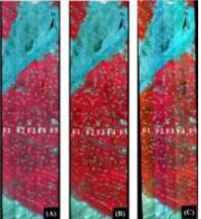
NBAR mosaics derived using local BRDF coefficients, NBAR mosaics derived using both of local and global BRDF coefficients and original CASI photograph mosaics were shown in the Figure 2. According to comparison of visual effects of BRDF correction for multiple-flightline aerial photograph mosaics, it could be concluded that BRDF effect was effectively removed using local and global BRDF coefficients calculated by the method proposed in this paper (Figure 2(B) and Figure 2(C)). The BRDF effects was not perfectly removed only using local BRDF coefficients (Figure 2(A) and Figure 2(C)). This shows that the use of the BRDF coefficients based on the method proposed in this paper produced good results. It should be noted that aerial images were mosaicked without using any image processing methods (histogram matching, color leveling, etc.) except for BRDF correction.

Figure 2. Visual effect of BRDF correction for multiple-flightline aerial photograph mosaics. (A) NBAR mosaics derived using local BRDF coefficients, (B) NBAR mosaics derived using both of local

and global BRDF coefficients, (C) original CASI photograph mosaics

Effect of BRDF Correction on Spectral Variations in the GSR

To illustrate the effects of BRDF correction on spectral variations in the CASI GSR, three plots (10m×10m) with different surface types were selected in the overlapped area of CASI flightline 1 and flightline 2, and the spectra of three surface types acquired from flightline 1 and flightline 2 before and after BRDF correction were compared, as illustrated in the Figure 3. It can clearly be seen from Figure 3 that the BRDF effects caused by different observing angle for the three surface types are significant, and the BRDF effects are strongly reduced for the three surface types across the full spectral range by BRDF correction. The effect of BRDF correction for maize is better than that for tree probably as a result of tree shadows. The effect of BRDF correction for desert is also significant.

Comparison of Correction Effects from Three Different Methods

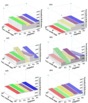
Figure 4. Linear regression trend of NBAR at 812 nm corrected to a fixed solar angle (SAA = 148.7°, SZA = 17.7°) for five aerial flightlines using three different methods. a1, a2 and a3 represent, respectively, the variation trends of NBAR derived using ‘one-step’ local parameters, ‘one-step’ global parameters and

‘two-step’ parameters for non-vegetation; b1, b2 and b3 represent the variation trends of NBAR for vegetation. Each color represents different flightline.

reflectance acquired over five flight lines were corrected to the NBAR at a fixed solar angle (SAA = 148.7°, SZA = 17.7°) using three different methods: (1) ‘one-step’ local RLM coefficients for each individual flightline; (2) ‘one-step’ global RLM coefficients for all flightlines; and (3) ‘two-step’ RLM coefficients proposed by this paper.

For the NBAR derived using the ‘one-step’ local RLM parameters, there are an insignificant change trend within flightline and a significant staircase change trend between flightlines (Figure 4 (a1) and Figure 4 (b1)). This demonstrates that the ‘one-step’ local RLM parameters are able to effectively simulate the anisotropic effects at the scale of a single flightline; however, because the ‘one-step’ local RLM parameters for a given flightline cannot be extrapolated to other flightlines, the ‘one-step’ local RLM parameters perform poorly when attempting to simulate the anisotropic effects across multiple flightlines.

For the NBAR derived using the ‘one-step’ global RLM parameters, there is an insignificant staircase change trend between flightlines and a significant change trend within flightline (Figure 4 (a2) and Figure 4 (b2)). This indicates that the use of ‘one-step’ global RLM parameters does not apply well to individual flightlines; however, this method is able to correct for the overall anisotropic effect between flightlines.

For the NBAR derived using the ‘two-step’ RLM parameters and correction algorithm proposed in this paper, there is an insignificant staircase change trend between flightlines (Figure 4 (a3) and Figure 4 (b3)). At the same time, the variation trends of the NBARs for all individual flightline are observed to be insignificant completely.

CONCLUSIONS

The acquisition of multiple-flightline aerial images covering a large area is required in many aerial remote sensing applications. However, the intrinsic observing characteristics of airborne sensors prevent precise comparison both within and between images due to BRDF effects 4-5. Therefore, BRDF correction for multiple flightline-aerial images is urgently needed for accurate, quantitative applications. In this paper, a new ‘two-step’ BRDF correction method based on the semi-empirical kernel-based model (Ross-Li model) was proposed as this model is able to explain the physical meaning of the BRDF effect. ‘One-step’ local RLM parameters for each individual flightline and ‘one-step’ global RLM parameters for all the flightlines together were also estimated using the BRDF fitting method based on the land-cover type, and different BRDF fitting effects and NBAR derived from different methods were compared.

geometry. In mathematics, the flow of this methodology makes the simulated surface reflectance more close to the original surface reflectance over multiple-flightline. And it is much easier to achieve high-accuracy simulation in each part, consequently, the simulation accuracy of arbitrary viewing/illumination reflectance could be improved. Therefore, ‘two-step’ correction method could obtain a high-quality NBAR for the case of multiple-flightline aerial images.

ACKNOWLEDGEMENT

The authors gratefully acknowledge the financial support provided for this research by Fund of development on science and technology Yellow River Institute of Hydraulic Research science and technology foundation programme (HKF201602), the National Natural Science Foundation of China (41325004), They also acknowledge the help of all the contributors to the Heihe Watershed Allied Telemetry Experimental Research (HiWATER).

REFERENCES

1. Kittilsen, P., H. F. Svendsen. 2004. “Three-level mass-transfer model for the heterogeneous polymerization of olefins,” J. Appl. Polym. Sci., 91: 2158-2167.

2. Goetz, F. H. 2009. “Three decades of hyperspectral remote sensing of the Earth: A personal view,”

Remote. Sens. Environ., 113:S5-S16.

3. Liang, S.L., H.L. Fang, and M.Z. Chen, et al. 2002. “Validating MODIS land surface reflectance and albedo products: Methods and preliminary results,” Remote Sens. Environ., 83:149-162.

4. Asmat, A., E. J. Milton, and P. M. Atkinson. 2011. “Empirical correction of multiple flightline hyperspectral aerial image mosaics,” Remote Sens. Environ., 115(10):2664-2673.

5. Beisl, U., and N. Woodhouse. 2004. “Correction of atmospheric and bidirectional effects in multispectral ADS40 images for mapping purposes,” Proceeding of the 20th ISPRS Congress, Istanbul, Turkey, IAPRS (ISSN: 1682-1750), 21, July 12-23.

6. Schiefer, S., P. Hostert, and A. Damm. 2006. “Correcting brightness gradients in hyperspectral data from urban areas,” Remote Sens. Environ., 101(1):25-37.

7. Kennedy, R. E., W. B. Cohen, and G. Takao. 1997. “Empirical methods to compensate for a view-angle dependent brightness gradient in AVIRIS imagery,” Remote Sens. Environ., 62(3): 277-291.

8. Beisl, U. 2002. “A new method for correction of bidirectional effects in hyperspectral imagery,” in

Proc. SPIE-Remote Sensing for Environmental Monitoring, GIS Applications and Geology, 45: 304-311.

9. Weyermann, J., A. Damm, and M. Kneubuhler, et al. 2013. “Correction of Reflectance Anisotropy Effects of Vegetation on Airborne Spectroscopy Data and Derived Products,” IEEE Trans. Geosci. Remote Sens., 52(1):1-12.

10. Collings, S., X. Wu, P. Caccetta, and N. Campbell. 2010. “Techniques for BRDF correction of hyperspectral mosaics,” IEEE Trans. Geosci. Remote Sens., 48(10):3733-3746.

11. Li, X., G. Cheng, and S. Liu, et al. 2013. “Heihe Watershed Allied Telemetry Experimental Research (HiWATER): Scientific objectives and experimental design,” B. Am. Meteorol. Soc., 94(8):1145-1160.

12. Wu, X. 2006. “Radiometric calibration of digital aerial imagery,” in Proc. 13th Australasian Remote Sens. Photogramm. Conf., Canberra, Australia.