Analysing and evaluating a dual sensor autofocusing method for measuring the position of patterns of small holes on complex curved surfaces

Analysing and evaluating a dual-sensor autofocusing method for

measuring the position of patterns of small holes on complex curved

surfaces

Xiaomei Chen*, Andrew Longstaff, Simon Fletcher, and Alan Myers, University of Huddersfield, Queensgate, Huddersfield HD1 3DH, United Kingdom * [email protected]. Tel: +44 1484 473844; Fax:+44 1484 472161

This paper proposes and discusses an active dual-sensor autofocusing method for measuring the positioning errors of arrays of small holes on complex curved surfaces. The dual-sensor unit combines an optical vision sensor and a tactile probe and is designed to achieve rapid automated measurements in a way that can be adapted to be suitable for deployment on a manufacturing machine tool. Mathematical analysis is performed to establish the magnitude of the deviation from the optimal focal length that is induced by the autofocussing method. This evaluation is based on the geometrical relationship and interaction between the radius of the tactile probe with both the measured holes and the complex-curved surface. A description is provided of a laboratory-based standalone dual-sensor autofocusing unit and test rig that was built to perform experimental validation of the method. This system is estimated to have a focusing uncertainty of 11 µm deriving mainly from the inaccuracy of the X-Z translation stage and the maximum permissible error of the tactile probe.

A case study is presented which evaluates the accuracy of a pattern of Ø 0.5 mm small holes on an elliptic cylinder. A mathematical analysis of that problem and practical results from both the tactile and optical sensors are provided and discussed. It is estimated that the deviation in optimal focusing induced by this automated method is between -23 µm and +95 µm. This is sufficiently accurate to ensure that the optical device can capture the entire space outline of each of the small holes on the complex curve surface clearly and can therefore identify its centroid from the image to provide a measurement of the position.

Keywords: autofocusing, tactile probe, optical vision sensor, position error, imaging processing.

Nomenclature

a,b Major radius and minor radius, respectively (mm)

CAD Computer aided design

CCD Charge coupled device

d Horizontal distance between dual sensors (mm) DCT Discrete cosine transformation

DOF Depth of field (µm)

OEF Optical evaluation function

L Vertical distance between forefronts of two sensors (mm) L0 Object distance of optical microscope (mm)

R,r Radii of tactile sensor and small hole, respectively (mm) uc(f) Positioning uncertainty of the testing rig (µm)

XOZ Measurement coordinate system

xoz Coordinate system of the workpiece

(Xi, Yi) Image centre of nominal hole in CCD panel (pixels)

(Xi′,Yi′) Image centre of drilled hole in CCD panel (pixels)

(Yi- Yi′) Centroid position change in axis (pixels)

∆z Focusing error caused by tactile probe radius (µm)

∆z′ Focusing error caused by position error of small hole (µm)

1. Introduction

The inspection and measurement of small holes on complex curved and freeform surfaces is a demanding problem in precision manufacturing. Such surfaces are commonplace within the automotive, aviation and space industries, where cooling holes with diameter less than Ø1 mm are commonly found. One type of aero-engine blade is designed with arrays of 79 air-cooling holes of Ø 0.3 mm and Ø 0.5 mm that need to be orientated within ±11 arc minutes. The latest generation of aero-engine blade has as many as 470 such small holes that need to be positioned accurately.

Measurement of such a large number of small features is impractical, if not impossible, using standard tactile probes that are commonly mounted on a coordinate measuring machine (CMM) or a computer numerical control (CNC) machine tool. Other probes that are designed for nano- and micro-metrology [1], especially the tactile optical-fibre probe [2] for the measurement of the diameter of small holes, are too fragile and costly to measure such a large number of small holes in a production environment.

An optical vision sensor that consists of a high-resolution digital camera and an optical microscope (a set of microscopic objective lenses) allows such measurements to be performed by means of image processing and vision inspection. This technology is broadly applied in various contour-related metrology fields, such as the inspections and measurements of hole orientation and position [3,4] on regular geometric shapes and surfaces of equal curvature such as a flat, a circular cylinder, a sphere, etc.; the form and profile of a workpiece [5,6]; the discovery and measurement of the surface defects [7]; wheel steer angle detection [8]; etc.

A clear image is necessary when using an optical vision system for measurement and inspection. Autofocussing is essential for efficient measurement and repeatable results. The autofocusing techniques currently used mainly rely on the various optical evaluation functions (OEFs) [9-11]. In practise, the optical microscope is driven to move from a short distance below the focal plane to a short distance above the focal plane while a series of images are captured at different planes. The corresponding series of OEF values are calculated and the plane whose image corresponds to the maximum of the OEF is approximately the focal plane. The procedure uses a hill-climbing search algorithm [12] that is ultimately limited by the resolution of the separation of the planes. The evaluation functions and algorithm are not mathematically complicated, and no additional hardware is required. CMMs equipped with an optical vision sensor usually employ such autofocusing methods.

2. Problem of single optical vision sensor autofocusing

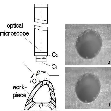
Fig.1. Ambiguity by only optically focusing the small hole on an engine blade surface at lens position C1 and C2:

corresponding images 1 and 2 are blurred in upper/lower semicircle and clear in the opposite semicircle.

An example of the limitations of OEF-based autofocussing is the inspection of a small hole on a turbine blade. The light-reflecting condition on the surface of the turbine blade introduces a significant level of noise, while the illuminating light reflects at different angles along the surface depending upon the curvature at each point. The OEF-based autofocusing method can find false solutions, as shown in Fig.1, where ambiguity exists while autofocussing on the outer border of a small hole drilled on the more skewed slope of the blade. If the optical microscope lens moves vertically to position C1, the lower half of the ellipse image is clear and upper half of it

blurs; if the optical microscope lens moves vertically to position C2, the upper half of the ellipse image is clear

while the lower half of it blurs. Between positions C1 and C2, the location of the focal plane is uncertain, with the

uncertainty increasing as the steepness of the slope increases.

Fig. 2. Focusing curves based on image DCT evaluation function for a hole on an elliptic cylinder shell under different

illuminating light intensity (LI) and a hardness indentation on a flat workpiece.

starting from beneath the focal plane, through the focal plane, then stopped above the focal plane. The ideal “focusing curve” versus “lens position” should have single peak with two mathematically monotonic sides; the steeper the side is, the higher the focusing resolution is and so the sharper the image contrast [15].

Since the DCT evaluation function was found to be the most capable focusing evaluation function among the others, it is taken as the example to explain the problem of autofocusing by using a single optical vision sensor based on the OEF. A series of images were taken at 5 µm intervals by the microscope lens with an approximate 100 µm DOF. The focusing values of the DCT evaluation function responding to the different images were calculated at each position and are plotted in Fig. 2. The starting vertical positions in Fig.2 are different for the elliptic cylinder with holes and the flat workpiece with a hardness indentation because the two workpieces are not at the same height. Therefore, Fig.2 was drawn such that the vertical position of an image whose DCT value is the maximum is considered to be approximately the true focal plane and is chosen as the zero microscope lens position. Consequently, the other vertical positions of the images either higher or lower than this zero are presented as negative or positive positions respectively. The DCT curve for the hardness indentation on the flat workpiece appears much sharper than holes on the elliptical cylinder.

3. Dual-sensor-autofocusing

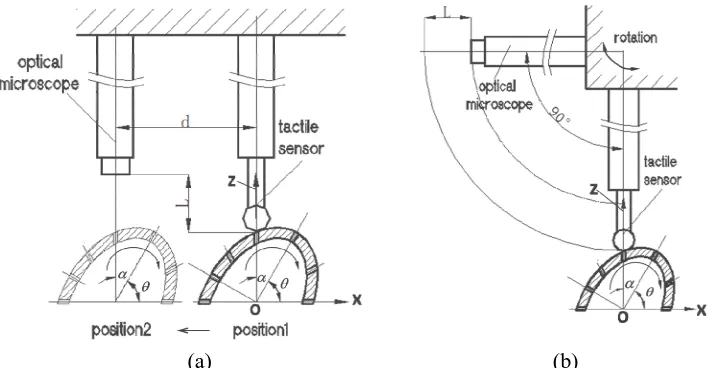
In consideration of the problems associated with OEF-based focusing, this paper proposes an active and fix-focusing method for the automatic measurement of the positions or orientations of arrays of small holes on the complex curved surfaces. The system works by combining an optical vision sensor and a tactile probe. The tactile probe locates the position of each of the small-holes in its sensing direction and feeds back the required offset to the actuator for the optical vision sensor, which can then position it to the required focusing position. A prerequisite for the dual-sensor autofocusing method is prior knowledge of the focal plane of the optical microscope, which can be found from its technical specifications or practical testing. The principle is that the distance L between the point of measurement of the tactile probe and the lens of optical microscope must be a known amount from the object distance LO of the optical microscope. In practice, it is most efficient to set L equal to LO. Two sensors must be assembled into one holder either parallel to each other with a known distance equal to d as shown in Fig. 3 (a) or perpendicular to each other as shown in Fig. 3 (b). The perpendicular configuration requires a rotary axis to swap between the two sensors.The XOZ in Fig.3 is the measurement coordinate system in the plane of the displacement of the two sensors. In this plane the sensors are either displaced (parallel configuration) or swapped (perpendicular configuration). The XOZ system takes the rotary stage centre as the coordinate origin for that plane, which is coincident with that of the workpiece. The Y-axis is perpendicular to the other two axes to complete the Cartesian coordinate system. All the holes can be sequentially measured by tactile probe in the first operation then optical vision sensor in the second operation (mode 1). Optionally, each hole can be alternately measured first by tactile probe and

second by optical vision sensor (mode 2).

Taking the parallel configuration in Fig. 3 (a) as an example, the procedure for measurement in mode 2 is as follows:

(1) One of the small holes is designated as the datum hole on the workpiece and is rotated by a rotary stage and/or translated by an x-axis stage to such a position that the central line of the datum hole aligns to the axis of the tactile probe;

(2) The tactile probe is translated downwards by the z-axis stage until the stylus contacts with the surface around the datum hole. A trigger signal is generated to cease the movement the stage as shown in Fig. 3(a), and the z-coordinate is measured as Z1;

or the workpiece is carried by an x-axis stage moving horizontally by a distance, d so that the datum hole is aligned by the optical microscope;

(4) The z-axis stage is moved downwards by a distance of |Z1-Z2| - (L - LO). The vertical distance L between the small hole and optical lens is equal to the object distance LO and the image of this small hole is clearly imaged onto the CCD panel and is captured by the CCD camera.

(5) After the image of the small hole is processed, the position of small hole is calculated based on the evaluation algorithms used for complex-curved surfaces.

(6) The workpiece is then repositioned and reoriented to locate the next small hole in the sequence according to the nominal CAD model. This process can be achieved automatically using an indexer or encoder feedback. (7) Steps 2 to 6 are then repeated until all the holes are measured.

(a) (b)

Fig. 3. Dual-sensor autofocusing configurations with (a) parallel and (b) perpendicular to each other, where L=L0.

Alternative dual-sensor measurement systems are commercially available. Some multi-sensor CMMs [2,12] are equipped with multiple z-axes that can load a tactile probe and an optical vision sensor simultaneously, in which case the dual-sensor autofocusing principle can be performed. A through-the-lens laser sensor [12] that is integrated with a coaxial optical vision sensor can switch between camera and laser, and more directly accelerate the focusing process than the dual-sensor autofocusing proposed in this work. However, the directional laser sensor will be deflected by the slope and skewness of the complex-curved surface. Such, laser range-finders are also adversely affected by surface properties, such as the low reflectivity of the surface of an aero-engine blade. Other commercially available multi-sensor CMMs have one z-axis and can load only one probe at a time.A single z-axis is a disadvantage for performing proposed dual-sensor autofocusing. A random positioning-error is introduced by homing, unloading one sensor and loading another sensor. The referring process takes time, yet cannot be omitted due to the default automatic measurement software.

4. Autofocusing deviations caused by probe radius and measured small hole

4.1. Small hole on protruding portion of a complex-curved surface

Ideally, the focal plane of the optical microscope should be on the same plane as the touch-point of the tactile probe. However, the spherical stylus tip of the probe will sink into the small hole by a depth s. s varies depending on the stylus radius in relation to the radius of the small hole under inspection as well as the curvature of the surface surrounding the hole. Consider the case of a small hole drilled near the top of a convex area or the bottom of a concave area. The influences of the radius of the tactile probe and the curvature of the complex curved surface on autofocusing accuracy are shown in Fig. 4.

If the radii of the tactile probe and small hole are R and r respectively, the stylus of the tactile probe is lower than the outline of the small hole by a distance of s, therefore

( )

s= −R R2−r2 R>r ₍₁₎ If the outline of a small hole on the complex-curved surface is not within one horizontal circle, but in a saddle or other loops, and if the height between the top point and bottom point is t, and the curvature radius of the complex-curved surface is ρ ,

( )

t= −ρ ρ2−r2 ρ>r (2)

Fig. 4. Schematic of a tactile probe contacting a small hole on the protruding part of a complex-curved cylinder.

Focusing errors (mm)

0.9

0 0.1 0.2 0.3 0.4 0.5 0.6 0.7 0.8

Radius r of small hole (mm)

1 0 0.1 0.2 0.3 0.4 0.5 0.6 0.7 0.8 0.9

R=0.25mm R=0.5mm R=1mm R=1.5

Focusing errors (mm)

1

0 0.2 0.4 0.6 0.8

Curvature radius p (mm)

10 0 1 2 3 4 5 6 7 8 9

r=0.1mm r=0.25mm r=0.5mm r=1.0mm

(a) (b)

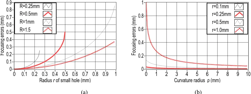
Fig. 5. (a) is the focusing deviation s versus radius of the small hole and (b) is the focusing deviation t versus curvature radius

of the complex curved surface.

different radii of the tactile probe R: 0.25 mm, 0.5 mm, 1 mm and 1.5 mm. Intuitively, these deviations will increase as the radius of the hole increases. To minimized s, the probe radius R should be as large as possible if the radius of the small holes is known. In Fig. 5 (b) focusing deviations (t) are plotted against the curvature radius of the complex-curved surface for different radii of the small hole (r): 0.1 mm, 0.25 mm, 0.5 mm and 1 mm. The focusing deviations t decrease with the increase of the curvature radius ρ. If the radius r, of the small holes is less than 0.5 mm, and the DOF of the optical microscope is in several hundreds micrometres, t can be considered insignificant.

4.2. Small hole on skewed and sloped portion of a complex-curved surface

The geometrical interaction between the spherical tip of the tactile probe and the complex-curved surface causes a probe deviation that varies according to the curvature of the contacted points on the surface. Following a detailed analysis of the geometrical relationship between the tactile probe radius R and the location at the complex-curved surface where a small hole with radius r is drilled with position error as shown in Fig. 6 (a) and (b), the focusing deviation formulas can be derived as follows.

(a) (b)

Fig. 6. Schematic of autofocus deviation caused by the tactile probe radius if it aligns on the complex-curved surface at (a)

the centreline of the hole and (b) offset from the centreline due to position error of the hole.

If a complex-curved surface implicitly expressed by F (x,y,z)=0 has continuous partial-differentiations to the variables x, y and z at point p (x,y,z), the normal vector n[17] at point p is

( , , ) ( , , ) ( , , )

( F x y z , F x y z , F x y z ) n

x y z

∂ ∂ ∂

=

∂ ∂ ∂ (3)

For a complex-curved surface which can be explicitly expressed by z = f (x, y), to set F (x,y,z)= f (x, y) - z, the partial differentiations in equation (3) are reintegrated as

( , , ) ( , )

( , , ) ( , )

( , , ) 1

F x y z f x y

x x

F x y z f x y

y y

F x y z z

_{∂ ∂}

= 

∂ ∂



∂ ∂



= 

∂ ∂



_∂

= − 

∂ 

(4)

( , )

( , )

f

x y

=

f x y

+ ⋅

R n

If γ represents the angle between the normal vector and Z-axis direction at p, its cosine is 1

2 2 2

( , ) ( , )

cos z ([ f x y ] [ f x y ] 1)

n x x

γ

∂ ∂ (6)

Therefore, equation (5) can be reintegrated as

( , )

( , )

/ cos

f

x y

≈

f x y

+

R

γ

If a small hole is drilled at the nominal position as shown in Fig. 6 (a), the position error of the small hole is zero so the centrelines of the small hole and the probe are coaxial. The autofocusing deviation caused by the probe radius is

( , )

( , )

(1/ cos

1)

E

z

f

x y

f x y

R

R

γ

∆ =

−

− ≈

−

Combining equation (6), (7) and (8), the autofocusing deviation caused by the probe radius is

2 1/2

[(tan

1)

1]

z

R

γ

∆ ≈ ⋅

+

−

where, 2 2 1/ 2

tanγ = ∂([ f x y( , ) /∂x] + ∂[ f x y( , ) /∂y] )

If the actual position of the small hole deviates from the nominal as shown in Fig. 6 (b), then the tactile probe will contact the surface either above or below the projected centreline of the hole. The diagram shows the case where the probe contacts the higher edge of the small hole. The linear position error of small hole, ∆l, causes an additional autofocusing error ∆z′. γ′is the slope at the point that where the surface intersects the Z-axis. Usually the probe radus R is much smaller than the curvature radius at the point p, γ′≈ γ. Therefore, the additional

autofocusing error ∆z′ is expressed as

∆z′ =∆l ⋅ tan γ′≈ r ⋅ tanγ (10) Ideally, to minimize the probing deviation ∆z, ∆z′ and R should be as small as possible in equation (9) and (10), respectively. It should also be noted that the probing deviation will increase as ∆l increases. Therefore, on poorly manufactured parts additional compensation of the focusing algorithm needs to be considered. The focusing deviations versus the slopes at the top edge of the small hole are plotted in Fig. 7. For the situation where the slope

around the higher edge of the small hole on the complex-curved surface, tanγ′ ,varies from 0° to 45° while the probe radius is 0.5 mm, 1 mm, 2 mm and 3 mm, respectively.

Focusing errors (mm)

1.4

0 0.2 0.4 0.6 0.8 1 1.2

skewness about hole centre (angle degree)

45

0 5 10 15 20 25 30 35 40

R=0.5mm R=1.0mm R=2.0mm R=3.0mm

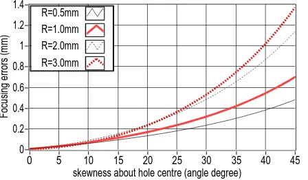
Fig. 7. Focusing deviations versus slope of the higher edge of small hole on complex-curved surface f (x,y) (∆l = r = 0.25 mm).

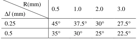
The focusing deviations increase with the increases of both the tactile probe radius and the slopes around the locations of the small holes on the complex-curved surface. The focusing deviations ∆z and ∆z′ need to be compensated if the radius is close to or larger than the DOF of optical microscope. This can be explained by considering an example of an optical microscope measuring system with 500 µm DOF. For different tactile probe radii of 0.5 mm, 1.0 mm, 2.0 mm and 3.0 mm, the focusing deviations ∆z and ∆z′ will reach the DOF if the skewed angle at the higher edge of a small hole on the complex-curved surface has reached the thresholds listed in table 1.

Table 1 Thresholds of skewed angles at the higher edge of a small hole on a complex-curved surface.

R(mm)

∆l (mm) 0.5 1.0 2.0 3.0 0.25 45° 37.5° 30° 27.5°

0.5 35° 30° 25° 22.5°

For an array of small holes on a complex-curved surface whose design parameters are already known, the probe radius should be chosen based on the comprehensive consideration of focusing deviation s, t and ∆z and ∆z′. They can be compensated by making an object-oriented-measurement strategy if the dual-sensor autofocusing unit is integrated into a high accuracy machine tool or a purpose-built test rig. Compensation can be made by correcting the deviation s, t and ∆z and ∆z′ from the height |Z1-Z2|. This means moving the optical microscope using the z-axis stage by a displacement L, calculated using equation 11, so that the related small hole can be clearly imaged by the optical microscope.

1 2

'

L

=

Z

−

Z

− + + ∆ + ∆

s t

z

z

5.1. An example of an autofocusing unit

Some types of CMMs that are equipped with two or more z-axes that can load an optical sensor and a tactile probe concurrently [2, 16] could perform the proposed autofocusing method, although it is unlikely that they could perform the automated method proposed without some hardware or software modification. If such a system is unavailable then a user-controllable dual-sensor autofocusing unit can be assembled. To validate the theory in this paper, such a system was built (Fig 8.).

The optical vision sensor comprised an optical microscope with tuneable magnification mounted with a coaxial LED ring light at its object end and connected to a CCD camera at its image end. The tactile probe could be a standard CMM or CNC machine tool probe. A contact inductive sensor (CIS) was used as the tactile probe for this test setup. The test rig had two linear (X- and Z-) axes and one rotary axis, which was employed to rotate the workpiece to each nominal angle of the small holes. The dual sensors were mounted onto the Z-axis. All axes were motorised to facilitate automatic focusing and measurement.

indirectly contribute to the positioning uncertainty. The remaining errors would influence the uncertainty of the position measurement of small holes. The test rig was not optimised for speed during these experiments, but it was fully computer-controlled to improve efficiency and repeatability. The CIS (GT21, TESA) has R 1.5 mm probe radius, 0.01 µm resolution and 0.2 µm maximum permissible error (EMPE) within 200 µm measuring range. The sensed voltage signal is output to TESATRONIC TT 60 electronic box and was digitally acquired by computer through a NI DAQ card. The optical microscope is an OEM product with 500 µm DOF and tunable optical magnifications. A rotary stage with 4.5 arc second resolution and 18 arc second positioning repeatability was mounted on the X-axis stage to rotate the workpiece for the following autofocusing experiment. The 11 µm positioning uncertainty contributed by the X-Z translation stage and maximum permissible error of the CIS is the result calculated by

2 2 2 2 2 1/2

( ) [2 2 ( ) ( ) ]

c r B PX BX MPE

u f = E + E +E d +E d +E (12)

where, EPX (d) = d × EPX =62.5×10/100=6.25 µm, EBX(d) = d × EBX ×(1/3600)×(π/180) = 4 µm and digit ′2′ means that the z-stage travels once forwards and once backwards.

(a) (b)

(c)

Fig. 8. Prototype dual-sensor autofocusing unit: (a) is its set-up, (b) is its kinematic schematic and (c) is a flowchart of

5.2. Focusing deviation caused by probe radius and the elliptic cylinder surface

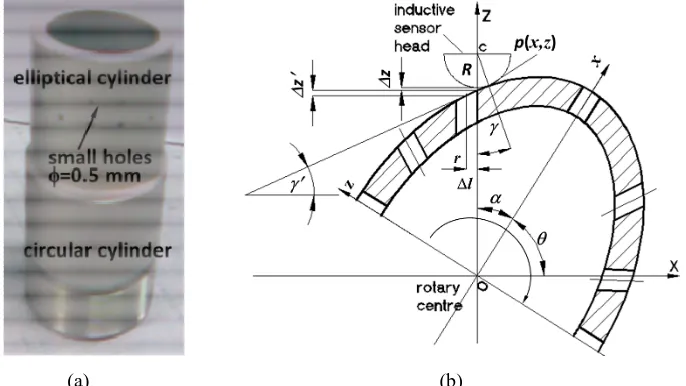
The autofocusing errors vary according to the different types of complex-curved surface. Therefore, a pattern of small holes on the circumference of an elliptic cylinder shell shown in Fig. 9 (a) is taken as an example to demonstrate how to analyse the autofocusing error.

(a) (b)

Fig 9.(a) Elliptic cylinder shell; (b) Schematic of an inductive sensor head contacting a small hole on an elliptic cylinder.

The schematic of the tactile probe contacting a small hole on the slope of the elliptic cylinder shell is shown in Fig. 9 (b). If xoz presents the workpiece coordinate system, the ellipse formula is

cos sin x a z b α α = ⋅   = ⋅

 (0≤α π<2 ) (13)

where, a, b are the major radius and minor radius of the ellipse respectively. The probe radius is R, and the small hole radius is r. The coordinate of the contact point in xoz coordinate system is (x, z). If the ellipse in the xoz coordinate system rotates an angle θ relative to the X-axis in XOZ coordinate system, the parametric function of the ellipse in XOZ coordinate system is expressed by

cos sin

sin cos

X x y

Z x y

θ θ θ θ = −   = + 

. (14)

If a small hole is contacted by the inductive sensor whose centreline is in the Z-axis, X=0. Thus, in equation (14)

cos sin

x θ=z θ (15)

If the hole drilled on the long axis is designated as the datum hole, α denotes the nominal angle of one of the other holes with reference to the datum hole and γ represents the angle between the normal vector and the Z-axis direction at p,

cos tan sin x a z b α θ α

= = ⋅ (16)

( / ) sin ( / ) cos

tan

( / ) cos ( / ) sin

dZ dx d dz d

dX dx d dz d

α θ α θ

γ

α ⋅ θ+ α ⋅ θ

= =

⋅ − ⋅ (17) Combining equation (16) and equation (17) gives

2 2

sin tan cos

tan sin(2 )

sin cos tan 2

a b a b

a b ab

α θ α

γ α

α α θ

− ⋅ + −

= =

− − ⋅ (0≤α π<2 ) (18)

2 2 2

2 1/ 2 2 1/ 2

2 2

( )

[(1 tan ) 1)] [(1 sin 2 ) 1]

4

a b

z R R

a b

γ − α

∆ = ⋅ + − = ⋅ + ⋅ − (19)

and

2 2

' tan sin(2 )

2 a b

z r r

ab

γ

α

∆ ≈ ⋅ = ⋅ (20)

If the first and second derivatives of the ellipse are dz dxand

2

2

d z

dx respectively, then

2

2 3 3

cot

sin dz b dx a

d z b

dx a α α = − =      (21)

The curvature of the ellipse is

2

2 3/ 2 2 2 2 2 3/ 2

2

(d z) / (1 (dz) ) / ( sin cos )

K ab a b

dx dx α α

= + = + (22)

Therefore, the curvature radius is

1 1 2 2 2 2 3/ 2

|K | (a sin b cos )

ab

ρ₌ − ₌ α₊ α ₍₂₃₎

R=1.5 mm. If r=0.25 mm, s ≈ 20 µm. If the small holes drilled at α = 45°, 135°, 225° and 315° are probed by the tactile probe, ∆z and ∆z′ reach their maximum. If the small holes drilled at α = 0°, 90°, 180° and 270° are probed by the same tactile probe, ∆z and ∆z′ diminish to their minimum. If a=14 mm, b=11.2 mm, the maximum and minimum focusing deviation ∆zmax=38 µm, ∆z′max=56 µm, ∆zmin=∆z′min = 0. If α = 45°, 135°, 225° and 315°, t ≈2 µm; if α = 90° and 270°, t ≈1.8 µm; if α = 0° and 180°, t ≈ 3 µm. When also considering the 11 µm autofocusing error introduced by positioning uncertainty uc(f) introduced by the test rig, the final focusing

deviation is between -23 µm and 95 µm, which are calculated by

2 2 2 1/2

min

2 2 1/2

max

[ ( )]

[( ') ( )]

c

c s t u f

z z u f

δ δ  _{= − + +}   = ∆ + ∆ +

 (24)

where, the negative and positive deviations mean that the optical vision sensor will over-focus and under-focus the small holes, respectively.

5.3. Autofocusing experiment

images marked with the detected centroids are shown in Fig. 10 (b). The procedure of autofocusing, image-capturing, image processing and centroid position detecting was conducted 5 times to evaluate repeatability. The measurement results are shown in Fig.11 (a) and (b), where the centroid deviations (Xi – Xi′) and (Yi – Yi′)

represent the deviation from the datum hole, located at 0°. The detailed centroid deviations and repeatability (σ) of 5 times measurement are listed in table 2. The largest non-repeatability takes place at the 120° hole, which is predicted to be caused by the imperfect of rotary stage and the assembled dual-sensor unit. Additional image-processing capability could be incorporated into the system to detect such artifacts automatically.

(a) (b)

Fig. 10. (a) Original images of a pattern of 12 small holes of Ø 0.5mm and (b) their binary images marked with the calculated centroids (3.75 times in optical magnification).

coordinates change (um)

100

-500 -400 -300 -200 -100 0

norminal hole positions (angle-degree)

360

0 50 100 150 200 250 300

round2 round3 round4 round5 round1 centroid deviations (Xi-Xi')

coordinates change (um)

140

-20 0 20 40 60 80 100 120

norminal hole positions (angle-degree)

360

0 50 100 150 200 250 300

round2 round3 round4 round5 round1

centroid deviations (Yi-Yi')

(a) (b)

Fig. 11. Repeatability of detected deviations of hole centroid in directions of (a) circumference (Xi – Xi′) (µm) and (b) axis (Yi – Yi′) (µm).

Table 2 Repeatability (σ) of detected deviations of hole centroid in circumference and axis direction. (Xi – Xi′) (µm) (Yi – Yi′) (µm)

Holes 1 2 3 4 5 STD 1 2 3 4 5 STD

0 0 0 0 0 0 0 0 0 0 0 0 0

30 -41.98 -40.60 -40.51 -40.93 -41.98 0.73 42.57 43.29 43.61 42.99 42.57 0.46

60 -374.43 -373.60 -374.27 -373.38 -374.43 0.50 71.67 71.83 72.13 71.60 71.67 0.22

90 -447.51 -456.96 -440.10 -455.50 -447.51 6.85 81.57 84.22 78.87 83.66 81.57 2.11

120 -417.64 -376.69 -391.15 -371.14 -417.64 22.05 106.31 103.39 104.72 103.30 106.31 1.49

150 -301.04 -323.71 -300.69 -314.51 -301.04 10.48 120.19 123.74 120.86 122.04 120.19 1.51

180 -250.98 -243.83 -250.48 -249.39 -250.98 3.03 104.91 102.71 105.62 104.59 104.91 1.09

210 -310.01 -311.62 -310.13 -312.60 -310.01 1.18 89.19 89.13 89.81 88.80 89.19 0.37

240 -461.76 -468.09 -461.78 -465.51 -461.76 2.91 54.45 54.46 55.18 54.36 54.45 0.34

270 -486.24 -490.25 -488.32 -485.57 -486.24 1.94 8.97 10.51 10.39 8.79 8.97 0.85

300 -397.85 -374.62 -388.96 -400.46 -397.85 10.62 29.52 30.25 30.27 29.29 29.52 0.46

330 -219.29 -214.95 -208.90 -215.04 -219.29 4.27 24.24 24.93 26.02 24.87 24.24 0.73

6. Conclusion

The ability to measure the position errors of small features rapidly and automatically is highly desirable in precision manufacturing, especially in the aerospace sector, where large patterns of small air-cooling holes are typically found on complex curved surfaces.

The autofocusing dual-sensor method of measuring arrays of small holes on complex curved surfaces has been proposed. It uses a tactile probe to find the optimal distance between an optical vision sensor and the targeted feature automatically. The mathematical treatment and evaluation of measurement results highlights the important parameters that should be minimised to reduce the error in the autofocussing method. The results are very promising for adapting the method to a production environment, in particular to on-machine measurement.

This method has the added advantage that it can be applied even if the optical microscope has a very short depth of field (DOF); the focusing deviation can be adapted electrically and mechanically to compensate it. The method has no perceived disadvantages in terms of measurement time over current optical autofocusing methods, which are based on various optical evaluation functions (OEF). Such systems need many images to be captured against the lens positions around the focal plane. The time required for moving the microscope, autofocusing, image processing and parameter calculating for each captured image using OEF, takes approximately 15 seconds. Experiments have shown that employing the autofocusing dual-sensor method, which only requires a single tactile-probing cycle to establish focal length and a single optical vision sensor to perform measurement, does not increase this cycle time. It is estimated that performing the technique on a high precision CNC machine tool will greatly reduce this cycle time because of the superior control setup over the test-rig.

This paper is concerned only with the autofocusing technique. After autofocusing and image processing, the evaluation algorithms of the position deviation of the patterns of small holes, the analysis of the measurement uncertainty of the position error as well as the due consideration for the real-time on-machine measuring system, are the subjects of continued research.

Acknowledgements

The authors wish to thank the UK’s Engineering and Physical Sciences Research Council (EPSRC) funding of the EPSRC Centre for Innovative Manufacturing in Advanced Metrology (Grant Ref: EP/I033424/1). Many thanks also to Mr Wenjun Zhang from Changcheng Institute of Metrology & Measurement (CIMM) Beijing for his assistance with this project.

Reference

[1] A. Weckenmann, G. Peggs, J. Hoffmann. Probing systems for dimensional micro- and nano-metrology. Measurement

Science and Technology 17 (2006) 504-509.

[2] http://www.werth.de/en/unser-angebot/products/multisensor-cmms.html (2013)

[3] H. Cao, X. Chen, K.T.V. Grattan, and Y. Sun, Automatic micro dimension measurement using image processing methods,

Measurement 31 (2002) 71-76.

[4] Z. Fei, J. Guo, and C. Li, A new method for detecting the diameter and spatial location of tiny through-hole, Advanced

Materials Research 189-193 (2011) 4186-4190.

IEEE International Technology and Innovation Conference (2006) 656-661.

[6] H. P. Syahputra, T. J. Ko. Application of image processing to micro-milling process for surface texturing. International J. Prec. Eng. Manuf. 15 (2013) 1507-1512.

[7] A. Zhou, J. Guo, W. Shao, J. Yang. Multipose measurement of surface defects on rotary metal parts with a combined laser-and-camera sensor. Opt. Eng. 52 (2013) 104104.

[8] T. Shu, Y. Zheng, Z. Shi. Image processing-based wheel steer angle detection. J. Electronic Imaging. 22 (2013) 043005. [9] F. Shen, L. Hodgson, K. Hahn. Digital autofocus methods for automated microscopy. Methods in Enzymology. 414 (2006) 620-632.

[10] M. Yang, L. Luo. A rapid auto-focus method in automatic microscope. IEEE International Conference on Signal Processing (ICSP) (2008) 502-505.

[11] C. J. Kuo, C. Chiu. Improved auto-focus search algorithms for CMOS image-sensing module. Journal of Information Science and Engineering 27 (2011) 1377-1393.

[12] X. Qiu, and Z.Yang, Study on entropy function optimization problem in auto-focusing algorithm applied for radar

imaging,IEEE International Conference on Microwave and Millimeter Wave Technology (ICMMT) 4, 2055-2058 (2008).

[13] A. B. Mario, Á B Josué, A. Leonardo, and C.María, Fast autofocus algorithm for automated microscopes, Optical

Engineering 44 (2005) 063601.

[14] W. Chen, M. Er, and S. Wu, Illumination compensation and normalization for robust face recognition using discrete

cosine transform in logarithm domain, IEEE Transactions on Systems, Man, and Cybernetics, Part B: Cybernetics 36 (2006)

458-466.

[15] J. He, R. Zhou, and Z. Hong, Modified fast climbing search auto-focus algorithm with adaptive step size searching

technique for digital camera, IEEE transactions on Consumer Electronics 49 (2003) 257-262.

[16] http://www.optiv.net/Multisensor--Optical-Systems_583.htm (2013).

[17] A. Jeffrey, Mathematics for engineers and scientists, sixth-edition, Chapman & hall/CRC (2004).

Biography

Xiaomei Chen attained her BEng in precision mechanical instrumentation and MEng in automatic test, measurement and control from Harbin Institute of Technology (HIT) in China. Then she joined Changcheng Institute of Metrology and

Measurement (CIMM) Beijing, Aviation Industry Cooperation of China (AIVC) as an assistant engineer, engineer, then

senior engineer in research and development of metrology instruments on geometrical and mechanical quantities. She has

been working there for many years until she went to Physiklisch-Technischen Bundsanstalt (PTB), Germany in Aug 2008 as

a research assistant toward a PhD on Nanometrology in the surface metrology department. She earned Dr. Ing. degree on

Electrotechnik and Nanometrology from Technische Universität Braunschweig. She has worked for a year in EEIE

Department of City University London as an academic researcher. She had received training for one month in 2005 for

nanometrology and nano-measuring machine in SIOS Meβtechnik GmbH, Germany. She joined in University of

Huddersfield in June 2012 as a research fellow in manufacturing metrology.

Andrew Longstaff gained a BSc in mathematics at Edinburgh University and an MSc in “Engineering Control Systems and Metrology” at the University of Huddersfield. His PhD investigated methods of evaluating the positioning capability of

Cartesian and non-Cartesian machines, since then he has been heavily involved in the development of measurement methods

for machine tools. He has been involved in improving the performance of manufacturing machines by the creation and

integration of error compensation systems. He has worked as a research fellow on several UK-government and industry-funded

grants and has taken part in four major EU-funded collaborative research projects. He is now a Principal Research Fellow in the