Defect Detection of Mobile Phone Surface Based on Convolution Neural Network

2017 2nd International Conference on Manufacturing Science and Information Engineering (ICMSIE 2017) ISBN: 978-1-60595-516-2

Defect Detection of Mobile Phone Surface

Based on Convolution Neural Network

Ling Ma, Yue Lu, Xiao Fei Nan, Yu Min Liu and Hui Qin Jiang

ABSTRACT

Automatic surface defect detection of mobile phone in large scale needs to process high resolution images and handle various defects while achieving high accuracy rate. This study proposes a defect detection method based on convolution neural network (CNN). Firstly, the original surface image of mobile phone is obtained using industrial linear array camera. Secondly, the obtained images are automatically segmented into specified sizes by the proposed preprocessing step. Moreover, we design the CNN on basis of GoogLeNet network, which greatly reduces the number of parameters without compromising prediction rate. At last the designed CNN are trained and tested. The trained CNN can be combined with a sliding window technique to detect any ROI with size larger than 256×256 resolutions in the original images. The experimental results show that the defect detection rate of the designed CNN can achieve as high as 99.5%.1

INTRODUCTION

With increasing production volume and high quality requirement of smart phone, surface inspection becomes a challenging task. Traditionally, surface inspection is performed manually. In most cases, it is highly subjective and time-consuming. To overcome the limitations of human inspection, automated surface inspection (ASI) techniques are vital processes in manufacturing to assist or replace human decisions. As described by Xie [1], existing ASI methods can roughly be divided into four categories: statistical, structural, filter based and model based. These methods are primarily used to manipulate images to extract defect features, such as scratches in

steel surfaces. However, the extensively varying real-world situations (e.g., lighting, shadow changes and low contrast defects) will affect the detection accuracy. Our work [2] about surface defects detection in TFT-LCD is also depends on the threshold parameters for extracting defect features.

At present, the domestic mobile phone surface defect inspection industry is still in the stage of manual detection. The manual detection rate is about 80%.Traditional defect detection, such as Canny edge detection and Sobel edge detection are not suitable for this kind of mobile phone surface defects with complex small defect or low contrast defect.

To solve the above problems, this paper presents a method for detecting defects on mobile phone surface based on CNN. CNN is a deep learning method for image recognition, classification, segmentation and detection, which is developed on the basis of multilayer neural networks [3]. As CNN are capable of learning image features automatically, the proposed method works without the conjugation of techniques for extracting features. The experimental results show that the proposed method can detect effectively point and scratch defects on smart phone surface.

OVERVIEW OF THE CNN

Deep learning, especially convolution neural networks, has been paid more and more attention as the research focus of image detection and pattern recognition in recent years. The general CNN consists of Convolution layer, Pooling layer and Full connection layer (FC). The convolution layer is used to extract the image features, and the multilayer convolution layer is usually used to obtain the deeper feature map. The pool layer is used to compress the feature map and extract the main features, so as to simplify the computational complexity of the network. The role of the FC layer is to connect all the feature maps and send the output values to the classifier , such as the soft max classifier.

Unlike other common defect detection methods, CNN automatically learn the features of an image by constantly updating the weights of the receptive field and narrowing the bias. Stochastic gradient descent (SGD) using back propagation is considered the most efficient and simplest method of minimizing bias [4]. General SGD follows Equation (1), where Wj decreases along the negative gradient direction. And the SGD algorithm with the momentum is expressed in Equation (2), where the momentum ε and the learning rate α are used to update the speed υ. Equation (3) is used to update the weights. The network can be continuously adjusted by repeating the above process until the Equation (3) converges.

   





W j

j W LW x y

W

j ; ,

 





(1)

   





WjLW;x ,y

  







   _j

j W

W ₍₃₎

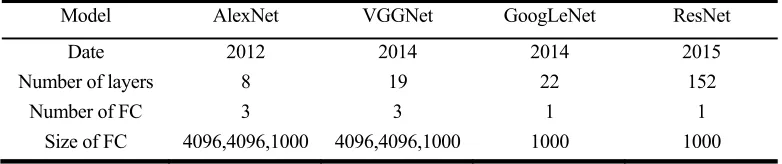
In the development of neural networks, several representative CNN are present. A classical CNN structure called AlexNet was proposed by Krizhevsky et al [5], and made a significant breakthrough in image recognition. VGGNet, GoogLeNet, and ResNet on the basis of AlexNet have achieved good performance in the ILSVRC competitions. It is generally believed that increasing the width and depth of the network is the most direct way to improve its performance [6]. TABLE Ӏ present the characteristics of several major CNNs . As we can see from TABLE Ӏ, with the development of CNNs, the number of layers and convolution kernels are increasing gradually, it also means a lot of parameters to be tuned, high computational cost, and tendency of over fitting. The fundamental solution to the above two problems is to convert all connected or even general convolution into sparse connected [7].

TABLE I. THECHARACTERISTICSOFSEVERAL MAINSTREAM CNN.

Model AlexNet VGGNet GoogLeNet ResNet

Date 2012 2014 2014 2015

Number of layers 8 19 22 152

Number of FC 3 3 1 1

Size of FC 4096,4096,1000 4096,4096,1000 1000 1000

Because the GoogLeNet network has designed and improved the inception module according to the Hebbian principle of biology[8], which can not only ensure the sparseness of the network, but also improve the computing performance. In order to avoid over fitting and shorter learning time in the case of learning large training samples, this paper selected GoogLeNet network and made some adjustments.

METHODS

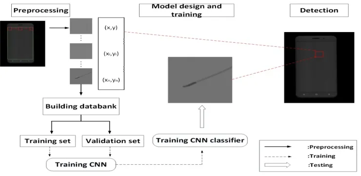
The proposed method includes three steps: Preprocessing, Model design and training, defect detection. The block diagram is shown in Figure 1.

Preprocessing

automatically segment the original images into sub-images of specified size, the coordinate information of the sub-images are also saved in the TXT document.

Figure 1. Block diagram of the proposed method.

Model Design and Training

Goog LeNet was designed by the Google team for the ILSVRC 2014 competition. The model consists of 22 layers, including1input layer,3convolution layers, 4 max pooling layers, 1mean pooling layer, 1FC layer, 3softmax layers and 9inception layers.

The GoogLeNet with sparse structure (inception layer) has better performance in extracting feature maps. To overcome the gradient vanishing problem, Goog LeNet skillfully adds two softmax layers at different depths to guarantee the disappearance of gradient return. Due to the nature of mobile phone surface and the defect is characterized by dots or lines, we removed the soft max layer of the Goog LeNet after the inception B and inception C layers, so the network can avoid overfitting while reducing the number of layers, and speed up training. The model diagram is shown in Figure2.

Figure 2. Schematic diagram of the model.

. Figure 3. Sample examples (a) Point defects, (b) Line defects.

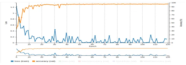
Figure 4. The result of training.

Defect Detection

In this paper, The test set containing 763images is fed into the trained CNN for classification. Each image is classified as 0,1, and 2 (i.e.no defects, point defects or line defects) by classifier. After the preprocessing step, the coordinate position of each test image is known. Through the sliding window technique, the original image is scanned and the coordinates of the classified images are positioned to the specific position of the mobile phone surface.

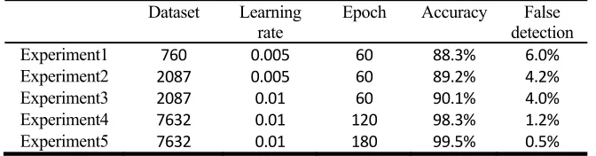
SIMULATION EXPERIMENT

Five experiments have been implemented with 763 test images. The experiment results are shown in TABLE ӀӀ. The accuracy are calculated by Equation (4). N0 are the number of no defect samples which are correctly detected, N1 are the number of point defect samples that have been correctly detected, N2 are the number of line defect samples which are correctly detected. Nt are the number of test set. The False detection rate is calculated by Equation (5). N0→1,2 are the number of samples that no defect samples were detected as defective samples and N1,2→0 are the number of samples that defective samples were detected as no defect samples.





A ₀ ₁ ₂ / ₍₄₎





F 01,2 1,20 / ₍₅₎

TABLE II. RESULTS OF FIVE EXPERIMENTS.

Dataset Learning

rate Epoch Accuracy detection False

Experiment1 760  0.005  60  88.3%  6.0% 

Experiment2 2087  0.005  60  89.2%  4.2% 

Experiment3 2087  0.01  60  90.1%  4.0% 

Experiment4 7632  0.01  120  98.3%  1.2% 

Experiment5 7632  0.01  180  99.5%  0.5% 

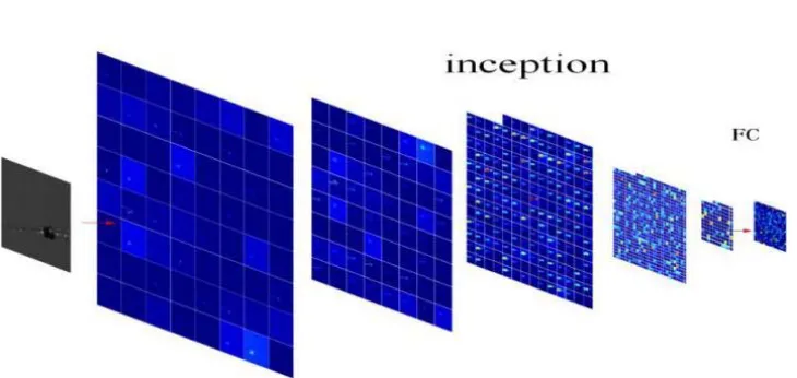
In order to analyze the correct and error detection samples, this paper selected two images for single test, and the test process is visualized, as shown in Figure 6.Aswe can see from the diagram, with convolution and pooling, the defect features of the test images are strengthened, and the features are obviously visible when passed through the inception layer. But the feature map of the error detection samples are not obvious as shown in Figure 7. This is because the defect has low contrast with small size.

Figure 5. The examples of error detection samples.

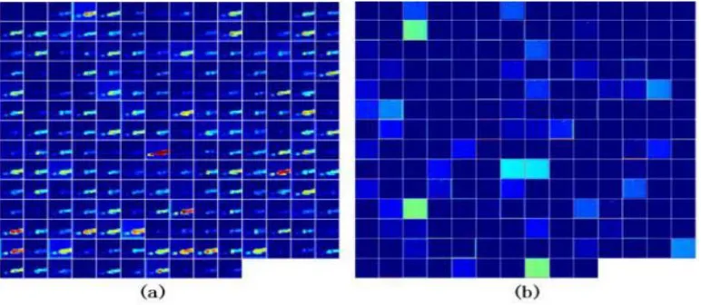
Figure 7. Inception layer contrast diagram for correctly detecting sample(a) and error detection sample(b).

As for defects on image edge, the input images become smaller while passing through the CNN, the defects on edges of the image have fewer chances to be recognized by the network than those in the middle of the image. In addition, some smaller and even invisible line defects of feature map are closer to point defects, which lead to detection errors.

However, defects at the edge of the image as in Figure 5 (c) (d) (e) (f)can be correctly detected in other sub images when scan ROI image with smaller slide than sub image size.

CONCLUSIONS

In this paper, a vision-based method for mobile phone surface defect detection has been proposed using the deep convolution neural network. The experiment results have shown that the proposed method has robust performance compared to traditional edge detection methods. Furthermore, the accuracy of the proposed method can achieve as high as 99.5%, and the false detection rate is 0.5%. The detection accuracy and detection efficiency are higher than the manual detection.

In the future, our research will focus on the improvement of the CNN to improve the detection performance and the detection of other defect types on the mobile phone surface.

ACKNOWLEDGMENTS

REFERENCES

1. X. Xie, “A review of recent advances in surface defect detection using texture analysis techniques,” Electron. Lett. Comput. Vis. Image Anal., vol. 7, no. 3, P1–25, 2008.

2. Ling Ma. Wei Liu. Huiqin Jiang, Yumin Liu. An Automatic Detection Algorithm for Surface Defects in TFT-LCD, 2nd ACPR2013, 5-8.

3. David Silver, et al. 2016, “Mastering the game of Go with deep neural networks and tree search.” Nature 529.7587 : 484-489.

4. LeCun, Y.A., Bottou, L., Orr, G.B. & Muller, K.-R. 2012. Efficient backprop, in G. Montavon, G.B. Orr, and K.-R. Muller (eds.), Neural Networks: Tricks of the Trade, 2nd edn., Springer,

Berlin Heidelberg, P9-48.

5. Krizhevsky, A., Sutskever, I. & Hinton, G.E. (2012), Image net classification with deep convolution neural networks, Advances in Neural Information Processing Systems, 1097-105.

6. Min Lin, Qiang Chen, and Shuicheng Yan. 2013. Network in network. CoRR, abs/1312.4400. 7. Sanjeev Arora, Aditya Bhaskara, Rong Ge, and Tengyu Ma. 2013. Provable bounds for learning

some deep representations. CoRR, abs/1310.6343.