S. N. Cresswell, T. L. McCluskey and M. M. West
School of Computing and Engineering, The University of Huddersfield, Huddersfield HD1 3DH, UK E-mail:{s.n.cresswell,t.l.mccluskey,m.m.west}@hud.ac.uk
Abstract
The problem of formulating knowledge bases containing action schema is a central concern in knowledge engineering for AI Planning. This paper describes LOCM, a system which carries out the automated generation of a planning domain model from example training plans. The novelty of LOCM is that it can induce action schema without being provided with any information about predicates or initial, goal or intermediate state descriptions for the example action sequences. Each plan is assumed to be a sound sequence of actions; each action in a plan is stated as a name and a list of objects that the action refers to.
LOCM exploits assumptions about the kinds of domain model it has to generate, rather than handcrafted
clues or planner-oriented knowledge. It assumes that actions change the state of objects, and require objects to be in a certain state before they can be executed. In this paper we describe the implemented
LOCM algorithm, the assumptions that it is based on, and an evaluation using plans generated through
goal directed solutions, through random walk, and through logging human generated plans for the game of Freecell. We analyse the performance of LOCM by its application to the induction of domain models from five domains.
1 Introduction
The area of Automated Planning Systems has progressed rapidly in the past 20 years. Planning algorithms have the ability to reason with knowledge of action and change in order to synthesise plans to achieve desired goals. The prevalent idea in Automated Planning research and development is that there is a logical separation of planning engine and domain model representing the application and problem at hand. However, these domain models are invariably hand crafted. As far as we are aware, all the domain models used in the International Planning Competitions (IPC) have been hand crafted, as are those reportedly used in leading applications such as those in the Space area.
Additionally we assume that there are many observations for it to use, and that the observations are sequences of possible action applications within the domain where each action application is made up of an identifier, and the names of objects that it affects.
LOCM works by assembling the transition behaviour of individual sorts, the co-ordinations between
transitions of different sorts, and the relationships between objects of different sorts. It does so by exploiting the idea that actions change the state of objects, and that each time an action is executed, the preconditions and effects on an object are the same. Under these assumptions, LOCM can induce action schema without the need for background information such as specifications of initial/goal states, intermediate states, fluents or other partial domain information. All other current systems e.g. Opmaker (Richardson (2008)), ARMS (Wu, Yang, and Jiang (2005)), and the system of Shahaf and Amir (2006) require some of this background knowledge as essential to their operation.
We evaluate the LOCM system with five domains: the tyre-world, the blocks world, driverlog, IPC Freecell and AoP-Freecell, with training sequences extracted from IPC solution plans, from using random walks generated using existing domain models, or from logs of human plans. The most impressive result is where LOCM creates a usable PDDL domain model from a number of logs of a human playing the Freecell game. This indicates the potential applications for such technology, where by observing logs of actions, agents with planning capabilities will be able to induce domain models in order to carry out planning themselves.
The paper is structured as follows. In the next section we describe the definitions and assumptions that underly LOCM and in doing so detail the steps in the LOCM algorithm. The following section details the evaluation with the five domains listed above. Finally, we detail similar and related work, outline future work and draw conclusions.
2 The LOCM System
2.1 LOCM Overview
The input to LOCM is an action training sequence, where each action is specified as a name followed by a sequence of affected objects. It is in a sufficiently general format that it could originate from a varied number of sources. The algorithm synthesises models in the form of Finite State Machines, and then augments FSM states with parameters which record associations between objects. The output is, for the purposes of this paper, a domain model in PDDL form. However, the internal representation would allow output in other forms such as SAS+(B¨ackstr¨om (1992)).
In this work we assume no prior knowledge of the planning domain theory: no information is given to the system about predicates, sorts, actions, goals, initial states, intermediate states etc - the only knowledge available is via the input training sequences. The only exception to this is the option to specify a “static” precondition, necessary in some domains which require static knowledge. Rather, we base our work on a set of assumptions or ontological constraints of the kind of planning domain theory being
learned. These assumptions are detailed below. Hence, although LOCM does not require other inputs,
it makes a fundamental assumption about the domain: that it consists of collections of objects (called sorts) which change state in such a way that this can be captured by parameterised finite state machines. The following subsections are motivated by examples in which we establish a conceptual framework of
definitions, assumptions and hypotheses. We use the heading of “ASSUMPTION” for facts about the
training sequence format and the domain’s structure. However these are independent of the content of the training sequences; we use the heading of “hypothesis” for knowledge that we induce from the content of the training sequence and hence the hypotheses are dependent on that content.
Example 1: Using the well known tyre-world as an example, the following is a action training sequence
containing ten action instances:
The intention is that c1, c2, c3 are containers (e.g. car trunks or boots), wr1, wr2 are wrenches, and j1, j2 are jacks, though the system is not given this knowledge.
The outline algorithm of LOCM is as follows: each line of the algorithm is detailed in the sections below.
procedure LOCM
Input: action training sequence Output: PDDL domain model
Step 1. Create sort structure and finite state machines
Step 2. Perform Zero Analysis and add new finite state machine if necessary Step 3. Create and test hypotheses for state parameters
Step 4. Create and merge state parameters Step 5. Remove parameter flaws
Step 6. Extract static preconditions (optional step) Step 7. Form action schemas
end
The output of LOCM (given sufficient examples) is a domain model consisting of sorts, object behaviour defined by state machines, predicates defining associations between sorts, and action schema in PDDL form. The action schema are induced having a fixed list of parameters, where each parameter ranges through objects belonging to some fixed sort.
2.2 Step 1: Induction of Finite State Machines
The input to LOCM is a training sequence ofNactions which all have the form: Ai(Oi,1, ..., Oi,m[i]) fori= 1, ..., N
whereAi is the action name, and this is followed by a list of object names of lengthm[i]. If objectOis
a member ofOi,1, ..., Oi,m[i], for some actioni, we say that the action containsO. Example 1 is such a training sequence, withN= 10,A1= open,A2= fetch jack, etc, andm[1] = 1, m[2] = 2, m[3] = 2,etc.
Definition: Universe of Objects
The set of objects in the domain is the set of all objects in the training sequence: OU={O:O∈Oi,1, ..., Oi,m[i], i∈1, .., N}
In Example 1,
OU={c1, j1, wr1, c2, wr2, j2, c3}
ASSUMPTION 1: Structure of the Universe
The Universe of objects is composed of a set of disjoint subsets, called sorts, such that:
– each object of each sort occupies a state which defines what is known about it at a certain stage of the changing world,
– objects of the same sort behave in the same way when acted on by actions, thus an action is associated with a single state. An example can be seen in Figure 1. However note that many actions can be associated with a single state.
– objects of the same sort can all be described by the same set of states.
ASSUMPTION 2: Consistency of Action Format
Givenith andjth distinct elements of the training sequence where namesA
i=Aj, thenm[i] =m[j],
and for eachk= 1, ..., m[i], objectsOi,kandOj,kshare the same sort.
Hypothesis 1: Sort Formation
The set of sorts which structure the domain are those obtained by applying Assumption 2 to every pair of actions with the same name in the training sequence.
Returning to Example 1, we can compute from it the hypothesis thatOU is composed of 3 sorts{c1, c2,
c3},{wr1, wr2},{j1,j2}.
Example 2: Consider the following extension to Example 1:
open(c1); fetch jack(j1,c1); fetch wrench(wr1,c1); close(c1); open(c2);
fetch wrench(wr2,c2); fetch jack(j2,c2); close(c2); open(c3); close(c3); close(wr1);
In this case, the final action close(wr1) would unite the container and wrench sorts into one, and OU
would be composed of 2 sorts{c1, c2, c3, wr1, wr2},{j1,j2}.
ASSUMPTION 3: States of a Sort
Theith actionA
i(Oi,1, ..., Oi,m[i])is assumed to cause (possibly null) transitions to allm[i]objects it contains. Theith action restricted to the single transition of thekth object,O
i,k, wherek∈1, .., m[i],
is calledAi.k. Each transitionAi.k, fori∈1, .., N andk∈1, .., m[i], moves an object of some sortG
between a start statestart(Ai.k)to a not necessarily distinct end stateend(Ai.k). Thus, transitions such
asAi.kform transitions of a finite state machine for each sortG.
Definition: Consecutive Actions
Assume that theithandjthactions from the training sequence contain a common objectOof sort G; that
isO=Oi,k=Oj,lfor somek, l. Then theithandjthactions are called consecutive with respect to object
O ifi < j, and nopexists,i < p < j, such that actionpcontainsO.
In Example 1,A1andA2are consecutive with respect to object c1.
ASSUMPTION 4: Continuity of Object Transitions
If theith andjth actions of the training sequence are consecutive with respect to an object O of sort G,
whereO=Oi,k=Oj,l for somek∈1, .., m[i],l∈1, .., m[j]; then the end state ofO’s transitionAi.kis
the same as the start state ofO’s transitionAj.l, that isend(Ai.k) =start(Aj.l).
Definition: Consecutive Transitions
The transitions Ai.k and Aj.l in Assumption 4 are called consecutive transitions in the finite state
machine associated withG.
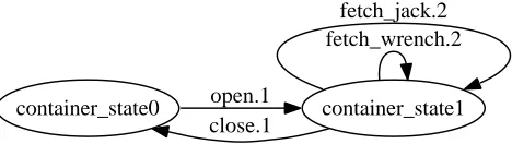
Returning to Example 1, consider transitions f etch jack.2 from action 2, and f etch wrench.2 from action 3, which both affect the same object c1. The actions are consecutive with respect to c1, hence end(f etch jack.2) =start(f etch wrench.2), andf etch jack.2andf etch wrench.2are consecutive transitions.
ASSUMPTION 5: Transitions are 1-1
If there are distinctith andjth actions in the training sequence such thatA
i=Aj, then for each pair
of transitionsAi.kandAj.k,k= 1...m[i],start(Ai.k)= start(Aj.k)andend(Ai.k)=end(Aj.k). In
other words, the name of each action restricted to any of its transitions forms a 1-1 map between object states.
Hypothesis 2: State Machine Formation
Consider objects of sort{c1, c2, c3} in Example 1. Focusing on the effect of the first four actions on object c1:
open(c1); fetch jack(j,c1); fetch wrench(wr1,c1); close(c1);
let us assign state namesS1, S2, .., S8to the input and output states of transitions affectingc1:
S1 =⇒open.1 =⇒ S2
S3 =⇒close.1 =⇒ S4
S5 =⇒f etch jack.2 =⇒ S6
S7 =⇒f etch wrench.2 =⇒ S8
Using Assumption 4 (continuity of object transitions) we can deduce thatS2=S5,S6=S7, andS8=S3. Taking into account the next four actions:
open(c2); fetch wrench(wr1,c2); fetch jack(j,c2); close(c2);
and Assumptions 4 and 5, we further deduce that S2=S7, S8=S5, S6=S3, and hence S2, S3, S5, S6, S7, S8all refer to the same state. Finally, utilising the last two actions
close(c3); open(c3);
We deduce thatS4=S1. Using the example training sequence with the Assumptions above, we have thus created an hypothesis for the behaviour of sort{c1, c2, c3}. This is meant to represent the sort container (such as the trunk or boot of a car - refer to Fig. 1).
container_state0 open.1 container_state1 close.1
[image:5.595.172.406.416.482.2]fetch_wrench.2 fetch_jack.2
Figure 1 FSM generated for the container sort
Algorithm for the induction of state machines:
Hypothesis 2, the assumptions above and the constraints that they entail leads naturally to an algorithm, used in Step 1 of LOCM to induce the Universe of each sort, and the state machines governing behaviour of the objects in each sort. The algorithm is described below in pseudo-code. In lines 1. through to 4., the set of states and transitions are built up. In lines 5. and 6., the continuity assumption is used to reduce the set of states by removing equivalent ones. At the end of Step 1, LOCM has induced a set of state machines, each of which can be identified with a sort, using Hypothesis 1.
Step 1
Input: action training sequence of length N Output: transition setT S, set of object statesOS 1. Initialise state setOSand transition setT Sto empty
2. Iterate throughAi, i∈1, .., N, andj∈1, .., m[i], as follows:
3. Add state identifiersstart(Ai.j)andend(Ai.j)toOS
4. AddAi.jtoT S
5. For each pair of consecutive transitionsT1,T2inT S
6. Unify statesend(T1)andstart(T2)in setOS
2.3 Step 2: Zero analysis
For some domains the induced domain model may be too permissive because the behaviour of an implicit
background object has not been captured. An example of this occurs in the AoP-freecell domain, a card
game in which there are separate pick-up and put actions. Without further analysis, the constraint that
pick-up and put actions must alternate is missing. The reason that this restriction would not be detected in
Step 1 above is that there is no single object named in the domain whose state indicates whether a pick or
put action comes next. The domain effectively contains an implicit hand object, which alternates between
an empty state and a holding state.
Strictly, this addresses a problem that is outside the scope of our assumptions, but the situation is common enough in extant domains that it is worth addressing. The state space of this kind of implicit object can be captured by assuming that every action has an implicit zeroth argument, which always refers to a dummy objectzero-object, i.e. For alli∈1. . . N, Oi,0=zero-object.
The algorithm of LOCM Step 1 is then repeated for the zero-object, and this results in a state machine. If the state machine for the zero object contains only one state, it is dropped and plays no further role. If the machine contains multiple states, then some information about the behaviour of an implicit object has been revealed, and this is Incorporated into the output PDDL domain. The zero state machine from the AoP-freecell domain is included in Fig. 9. The states of the zero machine give rise to predicates with no arguments in the output PDDL model.
We take the term zero analysis from a similar refinement in the TIM domain analysis tool (Fox and Long (1998)).
2.4 Step 3: Induction of Parameterised FSMs
Step 1 of LOCM creates a FSM for each sort found. States in a sort’s FSM capture state information about an object of that sort occupying the state. To capture relational information between objects, we let states be parameterised by the sorts of related objects. Here state parameters will record pairwise dynamic associations between objects.
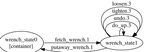
Consider the state wrench state0 for the wrench sort (Fig. 2). Considering the actions for
put-away wrench(wrench,container), and fetch wrench(wrench,container). For a given wrench, consecutive
transitions putaway wrench, fetch wrench, in any example action sequence, always have the same value as their container parameter. From this observation, we can induce that the state wrench state0 has a state variable representing container. The same observation does not hold true for wrench state1. We can observe instances in the training data where the wrench is fetched from one container, and put away in a different container.
[image:6.595.158.399.575.662.2]wrench_state0
[container] wrench_state1
fetch_wrench.1 putaway_wrench.1
do_up.3 undo.3 tighten.3 loosen.3
Figure 2 FSM generated for the Wrench sort.
hypothesise that there may be a relation between sortsGandG′. The hypothesis is retained if, for all
consecutive actionspandqin the training sequence with the names asB andC, we find that the same objectO′ of sortG′ appears in both, in the specified positions, that isO′=Op,k′=Oq,l′ (see diagram
below).
B(. . . , O, . . . , O′, . . .)
k k′
C(. . . , O, . . . , O′, . . .)
l l′
We formalise this as follows:
Hypothesis 3: Parameter Association
AssumeB.k andC.l are consecutive transitions in the FSM of sortG, and the actions with namesB andCcontain a parameter of a sortG′in positionsk′andl′respectively. Then we hypothesise that state
end(B.k)(=start(C.l)) has a parametric association of sortG′.
Example 3: Consider the training sequence:
open(c1); putaway jack(j1,c1); close(c1); open(c2); putaway jack(j2,c2); open(c1); fetch jack(j1,c1); fetch wrench(wr1,c1); fetch jack(j2,c2); close(c1);
From Step 1, we have transitionsB.k= putaway jack.1 andC.l= fetch jack.1 are consecutive, transitions to/from a particular state of the FSM for sort j1, j2. Both actions putaway jack and fetch jack share an argument of sort{c1,c2,c3}in position k′ = 2 andl′ = 2, so we hypothesise the state of a jack after
putaway jack.1has an association with the container sort.
Hypothesis Filtering
Assume we have a parameter match hypothesis specified by the values ofhS, B, k, k′, C, l, l′, G, G′i
as given above. Then consider all pairs of action at stepspandq, consecutive with respect to some object Oof sortGwhere
• Ap=BandAq=C,
• O=Op,k=Oq,l
If, for actionspandq,Op,k′6=Oq,l′, the hypothesis is falsified and removed from the set. Otherwise, the hypothesis is retained.
Returning to Example 3, we examine all pairs of actions which are consecutive with respect to some object in{j1,j2}. There are two pairs: the first pair is wherep= 2andq= 7. Here the actions in positions pandqare consecutive with respect to object j1, and there is an object (c1) which is of sort{c1,c2,c3}in both putaway jack(j1,c1) and fetch jack(j1,c1). The second pair is wherep= 5,q= 9. Here the actions in positionspandqare consecutive with respect to object j2, and there is an object (c2) which is of sort{c1,c2,c3}in both putaway jack(j2,c2) and fetch jack(j2,c2). Hence, in this training sequence, the hypothesis is retained.
Step 3
Input: action sequenceSeq, Transition setT S, Object setObs Output:HSretained hypotheses for state parameters
3.1 Form hypotheses from state machines
For each pairB.kandC.linT S
such thatend(B.k) =S=start(C.l)
For each pairB.k′andC.l′sharing sortG′ andk6=k′, l6=l′
Store in hypothesis setHSthe hypothesisH=hS, B, k, k′, C, l, l′, G, G′i end
3.2 Test hypotheses against example sequences
For each objectOoccurring inOu
For each pair of transitionsAp.mandAq.n
consecutive forOinSeq
For each hypothesisH=hS, B, k, k′, C, l, l′, G, G′i matchingAp=B, m=k, Aq=C, n=l
ifOp,k′=Oq,l′
then flagHas having a positive instance else removeHfrom hypothesis setHS endif
end end end
Remove any hypothesisHfromHSwithout a positive instance.
2.5 Step 4: Creation and merging of state parameters
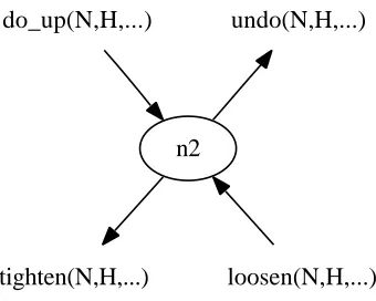
[image:8.595.195.365.535.671.2]Each hypothesis refers to an incoming and an outgoing transition through a particular state of an FSM, and matching associated transitions can be considered to set and read a parameter of the state. Since there may be multiple transitions through a give state, it is possible for the same parameter to have multiple pairwise occurrences.
Figure 3 shows an example of a state from the tyre-world for the sort nuts, with two incoming transitions and two outgoing transitions, with all of the actions involved having a sort hub for the second argument.
do_up(N,H,...)
n2
undo(N,H,...)
tighten(N,H,...)
loosen(N,H,...)
Figure 3 Part of FSM for sort nuts
hn2, do up,1,2, tighten,1,2, nuts, hubi hn2, do up,1,2, undo, l,2, nuts, hubi hn2, loosen,1,2, tighten,1,2, nuts, hubi hn2, loosen,1,2, undo,1,2, nuts, hubi
However, it is not appropriate to give staten2four separate parameters of sorthub— it should have only one. The first action of the pair in the hypothesis sets a state parameter. Wherever the same transitions occur as the first in the pair, they must set the same state parameter, regardless of the second in the pair.
Similarly, the second actions of the pair can be considered to read a parameter from the state. Wherever the same transitions occur as the second in the pair, they must always read the same state parameter, regardless of the first action in the pair.
These inferred equality constraints are used to reduce the set of parameters associated with each state. With each remaining hypothesish, we associate a parameterv, forming setbindingsof pairs ofhh, vi.
For any two pairshh1, v1iandhh2, v2i, such that: h1=hS1, B1, k1, k′
1, C1, l1, l1′, G1, G′1iand h2=hS2, B2, k2, k′
2, C2, l2, l2′, G2, G′2i then ifS1=S2,B1=B2,k1=k2andk′
1=k2′. we must enforcev1=v2- i.e. the parameters must be unified. Similarly, ifS1=S2,C1=C2,l1=l2andl′
1=l2′, we enforcev1=v2.
2.6 Step 5: Removing parameter flaws
A parameterP associated with an FSM stateS is said to be flawed if there exists a transition intoS which does not supplyP with a value. This means that an object can reach stateS withP having an indeterminate value. This may occur when there exists a transitionB.kwhereend(B.k) =S, but there exists nohsuch that:
h=hS, B, k, k′, C, l, l′, G, G′iandhh, Pi ∈bindings
For example, consider part of the FSM for sort hub in the tyre domain (Fig. 4). The actions do up and
undo both have an argument of sort nuts, and testing against example data retains the following hypothesis:
H0 =hhub2, do up,2,1, undo,2,1, hub, nutsi
This hypothesis says that wherever a hub undergoes a do up.2, and then its next transition is an undo.2 transition, then the nuts object referred to in the first argument of the do up action is the same as the object referred to in the first argument of undo action. In Step 4, we would create a parameterV0of sort nuts associated with state hub2 by a adding a bindinghH0, V0i.
hub2 [.., V0, ..] do_up.2
undo.2
jack_down.2 jack_up.2
Figure 4 Part of FSM for sort hub, with flawed parameter nuts.
However there is another transition jack up.2 which also leads to state hub2, and this transition does not occur in any corresponding binding which would link it toV0. Hence, there is a way to reach state
hub2 without providing a value for the parameterV0, so the parameter is flawed.
Step 5 detects and removes flawed parameters from the bindings set. The filtered set of bindings can then be used to generate state predicates for the output in a generated domain model.
2.7 Step 6: Extraction of static preconditions
to extract such static relationships in a fully automatic way, the information is often present in the training data and easy to extract.
An example from the freecell card game is that cards may only be placed in a homecell in the correct sequence - hence the relationship is a precondition of action put on card in homecell. In instances of this action, a successor relationship always holds between the first two arguments.
The difficulty lies in distinguishing relevant restrictions from irrelevant ones. So that the domain model can be completed with the relevant static conditions, LOCM has an option allowing the user to declare which arguments of which actions are subject to static restrictions. In LOCM+statics, this information is declared in the following form:
static( next(C1,C2), put_on_card_in_homecell(C2,C1,_) ).
These declarations are used in two ways:
• The relevant condition named in the first argument ofstaticis added as a precondition to the action in the second argument, with the variable bindings implied by the shared variable names.
• From the example sequences, matching instances of the action header are used to extract the set of static conditions which need to be declared in the initial state. This depends on the example data including at least one action depending on each static condition. For instance, if a training data sequences contains an action put on card in homecell(card 5 hearts,card 4 hearts,home 2), then we add a static fact next(card 4 hearts,card 5 hearts) to the initial state.
Unlike the core of LOCM, this process requires declared knowledge. In order to make clear the distinction, in the rest of the paper we refer to this knowledge-assisted part as LOCM+statics.
2.8 Step 7: Formation of PDDL action schema
Extraction of an action schema is performed by extracting the transitions corresponding to its parameters, similar to automated action construction in the Object Life History Editor (OLHE) process in Simpson, Kitchin, and McCluskey (2007). OLHE is a tool in GIPO III enabling action models to be defined by graphically constructing state machines. LOCM Step 7 creates one predicate to represent each object state. The output bindings from steps 3-5 above provides correlations between the action parameters and state parameters occurring in the start/end states of transitions. For example, the generated putaway wrench action schema in PDDL is:
(:action putaway_wrench
:parameters (?figure1 - wrench ?container2 - container) :precondition (and (wrench_state1 ?wrench1)
(container_state1 ?container2)) :effect (and (wrench_state0 ?wrench1 ?container2)
(not (wrench_state1 ?wrench1))))
The generated predicates wrench state0, wrench state1, container state1 can be understood as
in container, have wrench and open respectively. The generated schema can be used directly in a planner.
It would also be simple to extract initial and final states from example sequences, but this is of limited utility given that solution plans already exist for those tasks.
2.9 Use of the Domain Model in Planning Tasks
The solution we have adopted is to use actions to specify states. A direct analogy in the freecell domain is that the initial configuration of the cards is generated by dealing the cards using the actions
put in empty column and put on card in column. In doing so, we ignore the preconditions of the action,
and use only the end state of each object.
Similarly, the goal state can be specified by an action sequence using put in empty homecell and
put on card in homecell actions which simply deal cards into their desired final positions.
Thus it is possible to specify a planning task independently of the state representation.
3 Evaluation of LOCM
LOCM has been implemented in Prolog incorporating the algorithms detailed above. We have used LOCM
to create state machines, object associations and action schema comprising a domain model in PDDL for a range of domains. Here we attempt to analyse and evaluate it by its application to the acquisition of existing and new domain models. We used example plans from three sources:
• existing domains built using GIPO III (Simpson, Kitchin, and McCluskey (2007)): Tyre-world and Blocks World. In this case, we have created sets of example action sequences by random walk. A random initial state is generated, then the set of all actions that can be applied to that state is generated. Actions leading to a previously-visited state are filtered out. One of the action set is chosen at random, and then applied to the initial state to create a new state. The process continues, treating the new state as the initial state, until a predefined limit is reached, or no actions are applicable.
• domains which were used in the IPC3 planning competition1: Driverlog and Freecell. In this case, example training sequences extracted from the solution plans in the publicly released competition solutions have been used.
• logged events from a process: human players in Freecell. Freecell is a single player card game similar to the domain of the same name used in the IPC3 competition. It starts with the cards in a deck being randomly positioned in 8 columns face up. A player has to plan a sequence of card moves between freecells and card columns in order to leave all cards in 4 stacks in ascending order. We chose a particular implementation - AoP (Ace of Penguins) Freecell, and amended the code to log the card moves in the games played on it. Hence the action training sequences used were those that a human player generated in order to try to win the game from a random initial state.
3.1 Evaluation Criteria
Before stating evaluation criteria, we need to introduce some notation.
• Convergence: we introduce a type of convergence for the LOCM algorithm. We say that LOCM
converges after N steps if we can findNsuch that given a training sequence of length2N, it produces output from Steps 1–2 or Step 3 using the training sequence of lengthN, and produces no changes in its output from subsequenceN+ 1to2N.
• Equivalence: we introduce a type of equivalence between two planning domain models: an operator
set and an initial state< Ops1, Init1>are equivalent to< Ops2, Init2>iff the two directed graphs representing the space of reachable states are isomorphic (assuming edges are labeled with actions and the vertices (states) are not labeled).
• Adequacy: a domain model to be adequate if:
– where there is an existing domain model, we can determine that the induced model is equivalent to it, or contains redundant detail.
– where there is no existing domain model, given some initial state, the domain model permits all and only valid action sequences with respect to the context in the real world.
Our empirical evaluations were designed to explore the following criteria:
1
1. How many instances in a training sequence are required for LOCM to converge to a set of FSMs for each sort in the domain? How many instances in a training sequence are required for LOCM to converge to a set of parameterised FSMs for each sort in the domain?
2. Can LOCM produce an adequate domain model for test domains?
3. What difference do the different types of training sequence (generated by random walk with domain model; generated by planner with domain model; human-generated) make to the performance of
LOCM ?
4. What characterises the set of domain models that LOCM can learn?
We will comment on the first two criteria for each of the first four test domains below, and then comment on the second two criteria taking the test set as a whole. AoP-Freecell is used to test LOCM +statics.
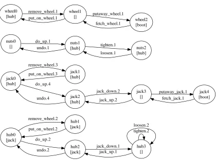
The Tyre-world (GIPO III version2). The input is a random walk training sequence. steps 1–2 converge
with a training sequence length of the order of N = 100, and step 3 with a length of the order of N = 2000. Figure 5, Figure 1 and Figure 2 illustrate the parameterised machines derived. An adequate domain theory is derived, which is equivalent to the domain theory used to generate the random walk sequence. The structural difference between generated and hand crafted domains is that the former contains extra states for the jack sort: when other parts of the assembly were changed (the wheel was placed on the hub, the nuts were screwed into the hub) LOCM designated a change of state for the jack. The extra states are redundant and hence do not compromise domain adequacy.
hub0 [jack]
hub1 [jack] remove_wheel.2
hub2 [jack] do_up.2
put_on_wheel.2
undo.2 jack_down.1jack_up.1 hub3[] tighten.2 loosen.2 jack0
[hub]
jack1 [hub] remove_wheel.3
jack2 [hub] do_up.4
put_on_wheel.3
undo.4
jack3 [] jack_down.2
jack_up.2
jack4 [boot] putaway_jack.1
fetch_jack.1 nuts0
[] nuts1[hub]
do_up.1
undo.1 nuts2
[hub] tighten.1
loosen.1 wheel0
[hub]
wheel1 [] remove_wheel.1
put_on_wheel.1 wheel2
[boot] putaway_wheel.1
[image:12.595.75.495.352.664.2]fetch_wheel.1
Figure 5 State machines generated for the tyre-world in addition to Figure 1.
The Blocks World (GIPO III version). The input is a random walk training sequence. steps 1–2 converge with a training sequence length of the order of N = 50, and step 3 with a length of the order of N
2
= 300. Figure 6 illustrates the parameterised machines derived. Here the block states correspond to the original as follows:
block0 - on a block and clear block1 - gripped by [gripper]
block2 - on a block and covered by [block] block3 - on table and clear
block4 - on table and covered by [block]
An adequate domain theory is derived, which is equivalent to the 6 operator domain theory used to generate the random walk sequence.
block0 []
[image:13.595.86.507.217.461.2] [image:13.595.197.389.608.666.2]block1 [gripper] grip_from_blocks.1
grip_from_one_block.1
block2 [block] put_on_blocks.3
put_on_blocks.1
put_on_one_block.1
block3 [] put_on_table.1
grip_from_blocks.3
grip_from_table.1
block4 [block] put_on_one_block.3
grip_from_one_block.3 gripper0
[block]
gripper1 [] put_on_table.2
put_on_blocks.2
put_on_one_block.2 grip_from_blocks.2
grip_from_table.2
grip_from_one_block.2
Figure 6 State machines generated for the blocks world.
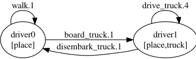
Driverlog (IPC PDDL-STRIPS version). The inputs are training sequences from the IPC archives. Steps 1–2 converge with a training sequence length of the order of N = 200, and Step 3 converges with a length of the order of N = 3000. Figure 7 illustrates the parameterised machines derived. The domain theory derived was not adequate in one respect: within the trucks machine, the distinction of states with/without driver is lost, and an extra state parameter (driver) is retained. The state machine for driver is shown in fig. 7.
driver0 [place] walk.1
driver1 [place,truck] board_truck.1
disembark_truck.1
drive_truck.4
Figure 7 Induced state machine for driver in driverlog domain.
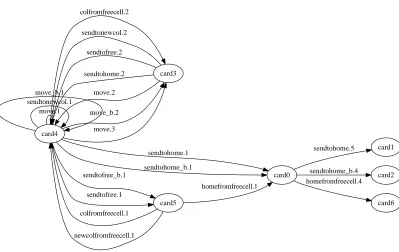
free columns. The state machine derived for the cards has 7 states. The states (see Fig. 8) can be understood as follows:
• card3 - in a column and covered by another card • card4 - in a column and not covered
• card5 - in a free cell • card0 - in a home cell
• card1, card2, card6 - in a home cell and covered
It is not helpful to distinguish the 3 final states, but LOCM cannot determine that they are equivalent. The domain theory derived is not adequate: whilst the LOCM results from Freecell are amongst the more interesting we found, there are a number of problems that LOCM version 1 is not equipped to handle:
• The distinction is lost between cards which are the bottom of a column and other cards which are in a column. Solving this problem requires weakening of the strong assumptions underpinning steps 1–2.
• LOCM does not automatically detect background relationships between objects— the
adja-cency of pairs of numbers, and the alternation of black cards on red cards. This problem is tackled is the next example.
card0
card1 sendtohome.5
card2 sendtohome_b.4
card6 homefromfreecell.4 card3
card4
sendtonewcol.2
sendtofree.2
sendtohome.2
move.2
sendtohome.1
sendtohome_b.1 colfromfreecell.2
move_b.2
move.3 move.1
sendtonewcol.1 move_b.1
card5 sendtofree_b.1
sendtofree.1
homefromfreecell.1
colfromfreecell.1
[image:14.595.93.492.339.591.2]newcolfromfreecell.1
Figure 8 Induced state machine for cards in IPC-Freecell domain.
AoP-Freecell
The AoP-freecell results are based on action traces collected by humans playing the game on a computer. An open source version of the freecell game3was modified in order to provide action traces,
which were then used to induce the planning model. The differences with the IPC freecell domain are:
• There are no sorts to represent the suit, colour or number of a card - the cards are only identified by unique object names.
3
• Instead of using direct move actions, there are separate pick-up and put-down actions. This reduces the total number of operators from 10 to 8.
• Freecells, homecells, and columns are each named objects. This is a much simpler and more natural approach than the IPC freecell, which uses a more sophisticated approach in which symmetries are eliminated by counting empty freecells, homecells and columns.
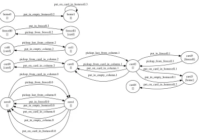
Using AoP-freecell action traces, LOCM induced a domain which was correct in its dynamic aspects. Because there is no named object which performs the pick-up and put-down actions, yet these actions always alternate, the zero analysis induces a 2-state machine.
However, the static relationships between cards are not detected, and to obtain these, we need to deploy
LOCM+statics (i.e. Step 6), which depends on a minimal declarative hint of three lines.
static( first(C1), put_in_empty_homecell(C1,_) ).
static( stackable(C1,C2), put_on_card_in_column(C1,C2) ).
static( next(C1,C2), put_on_card_in_homecell(C2,C1,_) ).
These correspond to three static predicates required in freecell:
first only aces may be placed into empty home cells,
next a card place on top of another card in a home cell must be of the same suit and of one value higher
than the card beneath it,
stackable a card stacked in a column must be of a different colour and one value lower than the card
beneath it.
From the example sequences, matching instances of the action header are used to extract the set of static conditions which need to be declared in the initial state. This leads to the following static conditions being extracted from the examples:
• 4 instances of first (complete - one for ace of each suit),
(first card_1_clubs) (first card_1_diamonds) (first card_1_hearts) (first card_1_spades)
• 48 instances of next (complete - 12 for each suit)
(next card_1_clubs card_2_clubs) (next card_2_clubs card_3_clubs) ...
• 88 instances of stackable (the complete set would comprise 96 instances, but whilst it is legal to place red/black ace on a black/red two, this is never useful, and so never occurs in the training data)
(stackable card_2_clubs card_3_diamonds) (stackable card_2_clubs card_3_hearts) (stackable card_3_clubs card_4_diamonds) ...
Hence, by deploying LOCM+statics with three lines of declared knowledge, the AoP-freecell was completed into a correct and usable planning domain. The resulting parameterised state machines are shown in Fig. 9.
Results Summary The size of the training sequence required for LOCM to converge for step 3 is
zero0 [] zero1 [] pickup_from_card_in_column.0 pickup_from_freecell.0 pickup_last_from_column.0 put_in_freecell.0 put_in_empty_homecell.0 put_on_card_in_column.0 put_in_empty_column.0 put_on_card_in_homecell.0 card0 [card] card1 [] pickup_from_card_in_column.2 put_on_card_in_column.2 card2 [] pickup_last_from_column.1 pickup_from_card_in_column.1 put_on_card_in_column.1 put_in_empty_column.1 card5 [freecell] put_in_freecell.1 card3 [home] put_on_card_in_homecell.1 put_in_empty_homecell.1 pickup_from_freecell.1 card4 [] put_on_card_in_homecell.2 col0 [card] col1 [] pickup_last_from_column.2 put_in_empty_column.2 freecell0 [] freecell1 [card] put_in_freecell.2 pickup_from_freecell.2 home0 [] home1 [] put_in_empty_homecell.2 put_on_card_in_homecell.3
Figure 9 Parameterised state machines for AoP-freecell
Addressing the third criteria, we note that randomly-generated example data can be different in character from purposeful, goal-directed plans. In a sense, random data is more informative, because the random plan is likely to visit more permutations of action sequences which a goal-directed sequence may not. However, if the useful, goal-directed sequences lead to induction of a state machine with more states, this could be seen as useful heuristic information. Where there is only one object of a particular sort (e.g. gripper, wrench, container) all hypotheses about matching that sort always hold, and the sort tends to become an internal state parameter of everything. For this reason, it is important to use training data in which more than one object of each sort is used, and this tends to favour the use of randomly-generated training sequences.
We now consider the fourth criterion - the class of domain theories that can be induced. From the Assumptions about the kind of structure we are expecting (in particular Assumption 3, which stipulates that transitions are 1-1), and from the empirical evaluation above, it follows that LOCM can induce adequate domain models for a restricted form of STRIPS. The type of training sequence is one that utilises more than one object of each sort. Assumption 3 implies that an action moves the objects in its arguments between clearly-defined substates. Objects which are passively involved in an action may make a transition to the same state, but cannot be in a don’t care state.
The main restriction is that static background information, such as the specific fixed relationships between objects (e.g. which places are connected), is not automatically analysed by the system. In general, this can lead to missing preconditions. The LOCM algorithm assumes that all information about an object is represented in its state and state parameters. In general, this form of information may vary between training examples.
4 Related Work
and Yang (2009)). This research is motivated in several ways: some argue that for intelligent agents to be able to adapt and plan in unseen domains, they must be able to learn a new domain model; others argue that correct domain models are impossible to know a priori, and agents must be able to incrementally adjust their existing model. Others use the less ambitious motivation that human-driven knowledge acquisition and maintenance requires automated support.
The area of process mining is a technique used in Business Process Management (BPM) which seeks to use events or logs recorded while a (business) process is being executed. The outcome is a business process model that would explain the logs. An example is provided by Hoffmann, Weber, and Kraft (2009) where work is described which induces a model which is then turned into a workflow. The focus of process mining research is on learning from sequences of events: for example, assuming an event alphabet of A, B, C, D, E, the input to the algorithm is a set of observations such as AABCA, ABCCAD, AEDDDCC etc. The process mining algorithms induce process models in the form of machines such as Petri Nets. This is similar to the machine learning area of grammar induction, and techniques seem to draw on this area. Process mining is more general in that it assumes that a sequence of concurrent processes causes the events, and therefore has to deal with concepts of process synchronisation.
The rationale for process mining is in part to help in the difficult problem of engineering a model and in this respect it is similar to that of learning action knowledge. However the results of learning are different from those used in AI Planning. In BPM the technique is used to aid the construction and analysis of a process model, whereas in Planning the results are input to a planning engine. Also, the induction of planning actions from traces is at a higher degree of granularity and requires stronger assumptions. An induced domain model will contain a model of objects, relations and attributes, in which the physics of actions are captured. Hence traces are also sequences of “events”, but events are action applications, and each is described in terms of a name and all the objects that are affected or are needed during the event. Then there is the assumption about objects having their behaviour described by a machine. The PDDL or OCL which is output by LOCM is more expressive than the kind of Petri Nets induced by process mining.
Learning STRIPS-type action schema has also attracted a large amount of research in recent years. Some systems learn from many plan examples with little background knowledge (e.g. the ARMS system of Wu, Yang, and Jiang (2005)). In contrast Opmaker learns from a single example together with a partial domain model. The Opmaker algorithm detailed in McCluskey et al. (2009); Richardson (2008) is one of a family of algorithms which commenced with McCluskey, Richardson, and Simpson (2002). Opmaker is described more fully in a Ph.D. thesis (Richardson (2008)), who also details how it is able to learn heuristics in the form of hierarchical action representations containing plan fragments. Each Opmaker system acquired knowledge from sequences of actions which, given an initial state, solve a given task. The system assumes knowledge of objects, object classes, domain constraints, and possible states of objects - collectively called static knowledge, or partial domain knowledge. For example, for each action in the sequence, it is known which object(s) change and which do not. In addition, domain invariants are provided which aid the production of unique action schemas.
Other systems require richer input: ARMS Wu, Yang, and Jiang (2005); Zhuo, Hu, and Yang (2009) makes use of some background knowledge as input, comprising types, relations and initial and goal states and also uses sets of examples. However ARMS takes a consistently predicate-centric view, unlike
Opmaker and LOCM which are object-centric. Learning in ARMS is statistical in nature, and outputs
a solution which is optimal with respect to reduced error and redundancy rates. The former is defined as the proportion of preconditions that cannot be established by any action in the previous part of the plan. The latter establishes the degree of redundancy created in the action model in the example set. The
Opmaker algorithm relies on an object-centred approach similar to LOCM, but it too requires a partial
do, however, use a richer representation for action schema. The TIM domain analysis tool (Fox and Long (1998)) uses a similar intermediate representation to LOCM (i.e. state space for each sort), but in TIM, the object state machines are extracted from a complete domain definition and problem definition, and then used to derive hierarchical sorts and state invariants.
Both LOCM and Opmaker use positive examples in the solution sequence. The Planning Operator Induction (POI) system of (Grant (1996)) learns from positive examples and uses a default rule to provide negative information which boosts the positive training instances. In more recent work (Grant (2007)), POI is extended to a multi-agent system. The work is based on representations of operators and constraints which between them model the domains, so the modelling process is fundamentally different from ours. The author presents a good assessment and diagrammatic model of planning in the case where an initially complete domain model is shown to be capable of receiving and assimilating sensory feedback. Because this initial domain model is distributed across several agents who, as a set, have complete knowledge, individual agents will have only partial knowledge and must share this knowledge for planning to be successful. The emphasis in Grant (2007) is on how the recipient agent assimilates the knowledge of another agent.
Learning expressive models from examples is a central goal in the Inductive Logic Programming community. In his thesis Benson (1996), reasons about TRAIL, which represents actions via
teleo-reactive (TR) programs. TR programs are durative rather than discrete. Benson describes an ILP method
for learning action schema in TRAIL, using background knowledge and multiple positive and negative training examples. Additional knowledge is provided in the form of mode definitions for predicates (i.e. input and output). Action schema are learned by transforming first-order instance descriptions to propositional form and using a method based on the FOIL algorithm of Quinlan (1990).
5 Conclusion
In this paper we have described the LOCM system and its use in learning domain information (comprising object sorts, state descriptions, state machines and action schema), and outputting usable PDDL domain models, when input with training action sequences. Characteristic of previous work in this area is that input to the learning process includes some planning oriented knowledge, such as state information, predicate descriptions, plan goals and initial state, etc., as well as the training data. For domains such as the tyre-world, LOCM learns an adequate model without any a priori domain specific knowledge. LOCM also learned an adequate domain model for the AoP Freecell game from training sequences obtained via logs of actual games, although in this case the system required the specification of three simple static preconditions.
We view LOCM as the first step in creating tools which can truly learn planning domain models by observing, without the need for human intervention or handcrafting. Results of our evaluation using five domain models show LOCM’s success, but also point to future work:
– although it is unrealistic to expect example training sequences to be available for all new domains, we expect the technique to be beneficial in domains where automatic logging of some existing process yields plentiful training data, e.g. games, workflow, or online transactions. We are currently building up an idea of the scope of such a tool within the context of the growing availability of online data;
– in the near future, we plan to develop LOCM in two directions (i) to give it the capability to develop sorts with objects that are described by more than one state machine. This would provide a elegant solution to domains such as driverlog, where objects have aspects that change subject to different state machines; (ii) to investigate the feasibility of learning static preconditions from the examples, rather than stipulating that they need to be given along with the training sequences;
References
B¨ackstr¨om, C. 1992. Equivalence and tractability results for SAS+planning. In Swartout, B., and Nebel, B., eds., Proceedings of the 3rd International Conference on Principles on Knowledge Representation
and Reasoning (KR-92), 126–137. Cambridge, MA, USA: Morgan Kaufmann.
Benson, S. S. 1996. Learning Action Models for Reactive Autonomous Agents. Ph.D. Dissertation, Dept of Computer Science, Stanford University.
Fikes, R.; Hart, P. E.; and Nilsson, N. J. 1972. Learning and executing generalized robot plans. Artif.
Intell. 3(1-3):251–288.
Fox, M., and Long, D. 1998. The automatic inference of state invariants in TIM. J. Artif. Intell. Res.
(JAIR) 9:367–421.
Grant, T. J. 1996. Inductive Learning of Knowledge-Based Planning Operators. Ph.D. Dissertation, de Rijksuniversiteit Limburg te Maastricht, Netherlands.
Grant, T. J. 2007. Assimilating planning domain knowledge from other agents. In Proceedings of the
26th Workshop of the UK Planning and Scheduling Special Interest Group, Prague, Czech Republic, December 2007.
Hoffmann, J.; Weber, I.; and Kraft, F. M. 2009. Planning@SAP: An application in business process man-agement. In Proceedings of the 2nd International Scheduling and Planning Applications woRKshop
(SPARK’09), at ICAPS’09.
McCluskey, T. L.; Cresswell, S. N.; Richardson, N. E.; and West, M. M. 2009. Automated acquisition of action knowledge. In International Conference on Agents and Artificial Intelligence (ICAART), 93–100.
McCluskey, T. L.; Richardson, N. E.; and Simpson, R. M. 2002. An Interactive Method for Inducing Operator Descriptions. In The Sixth International Conference on Artificial Intelligence Planning
Systems (AIPS), 151–160. AAAI Press.
Quinlan, J. 1990. Learning logical definitions from relations. Machine Learning 5:239–266.
Richardson, N. E. 2008. An Operator Induction Tool Supporting Knowledge Engineering in Planning. Ph.D. Dissertation, School of Computing and Engineering, University of Huddersfield, UK.
Shahaf, D., and Amir, E. 2006. Learning partially observable action schemas. In Proceedings, The
Twenty-First National Conference on Artificial Intelligence and the Eighteenth Innovative Applications of Artificial Intelligence Conference, July 16-20, 2006, Boston, Massachusetts, USA. AAAI Press.
Simpson, R. M.; Kitchin, D. E.; and McCluskey, T. L. 2007. Planning domain definition using GIPO.
Knowl. Eng. Rev. 22(2):117–134.
Wu, K.; Yang, Q.; and Jiang, Y. 2005. ARMS: Action-relation modelling system for learning acquisition models. In Proceedings of the First International Competition on Knowledge Engineering for AI
Planning.