A Relationship Function Between Loadability Margin and OMIB Simulation Results for Heavy Loading Power System

2018 International Conference on Modeling, Simulation and Optimization (MSO 2018) ISBN: 978-1-60595-542-1

A Relationship Function Between Loadability Margin and OMIB

Simulation Results for Heavy Loading Power System

Yu-long HUANG

_{and Ming-bo LIU}

1_{Institute of Rail Transportation, Jinan University, Zhuhai, China} 2_{Electrical and Information College, Jinan University, Zhuhai, China}

3_{School of Electric Power Engineering, South China University of Technology, Guangzhou, China} *Corresponding author

Keywords: Voltage stability, One-machine-infinite-bus equivalent, Loadability.

Abstract. A novel voltage stability relation function based on an one-machine-infinite-bus (OMIB) equivalent was proposed, which shows detailed relationship between voltage stability and transient stability. Since the OMIB hybrid simulation has the ability to take into consideration any kind of system detailed dynamic model, the proposed voltage stability relation function embodies all the system’s nonlinearity, which is stricter than traditional static voltage stability indexes. The feasibility and validity of the proposed index were demonstrated on 9-bus, 14-bus, 39-bus and 692-bus systems.

Introduction

Proximity of voltage instability is usually measured by the distance between the operating point on the PV curve and the limit of the same curve [1]-[3], i.e. system loadability margin. However, loadability margin analysis does not include the system detailed dynamic model, and may draw a false (un)stable conclusion when system operates near a critical stable operating point.

While one-machine-infinite-bus (OMIB) simulation can take into consideration any kind of system detailed dynamic model, i.e. system’s detailed nonlinearity. A relation function between loadability margin and OMIB simulation results is proposed in this paper, which shows detailed relationship between voltage stability and transient stability. Since OMIB hybrid simulation can use system detailed dynamic model, the proposed relation function embodies all the system’s nonlinearity, which is stricter than traditional static voltage stability indexes. The feasibility and validity of the proposed function are demonstrated on 9-bus, 14-bus, 39-bus and 692-bus systems.

OMIB Hybrid Simulation Method

Based on the extended equal area criterion [4]-[5], OMIB hybrid simulation methods based on time domain simulations are proposed in [6]-[8].

 

 

 

 

 

a r m r e r

r

o r

P t P t P t

t

t t t t

          _{   }  (1)

where P_a is the equivalent OMIB accelerating power, P_m is mechanical power, P_e is the electrical power, ˆ is the equivalent rotational speed deviation, to represents the initial time at which the

system is in steady state conditions (i.e. right before the fault), and t_r is the time at which the maximum oscillation equivalent angle ˆ_r is reached.

The “generally” unstable criterion is given by:

 

 

 

 

a u m u e u

a t t

o

P t P t P t

dP dt

t t t

   _{  }   _    _{  }  (2) 0 ˆ

 ˆc ˆr ˆu

ˆ  P s  e P m P

ˆ0 ˆc ˆu

ˆ 

P Pe

m

P

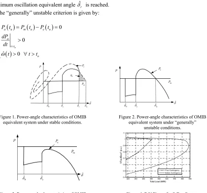
Figure 1. Power-angle characteristics of OMIB

equivalent system under stable conditions. Figure 2. Power-angle characteristics of OMIB equivalent system under “generally” unstable conditions.

0

ˆ

 ˆc

ˆ



P P_e

m P

320 340 360 380 400 420 440 460 480

0.4 0.5 0.6 0.7 0.8 0.9 1 1.1

Total Load (MW)

V F aul tB us7 ( p. u. ) Post Contingency Before Contingency

Figure 3. Power-angle characteristics of OMIB

equivalent system under “very” unstable conditions. Figure 4. P-V Figure for 9-Bus System after Disturbance.

This is depicted in Figure 2, where the OMIB trajectory reaches the unstable equilibrium ˆ_u point at time t_u after the fault clearance. The critically (un)stable trajectory evaluation criterion is given by:

 

 

 

 

0

ˆ 0

a a m a e a

a

P t P t P t

t



  



 _

 (3)

 

a

P t    t t t (4) where t_end is the total simulation time.

PV Curves of Four Test Systems

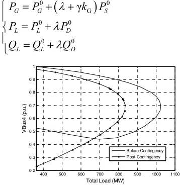
Proximity of voltage instability is usually measured by the distance between the operating point on the PV curve and the limit of the same curve, i.e. system loadability margin. So first of all, PV curves of four test systems, i.e. IEEE 3-machine 9-bus system, IEEE 4-machine 14-bus system, 10-machine 39-bus New England benchmark system, and a real provincial 138-machine 692-bus system, are computed by using CPF in PSAT [10] which can be seen in Figure 4-7. The continuation power flow (CPF) computations are performed considering voltage limits and reactive power limits for all the systems except 14-bus system in which only voltage limits are considered.

For 9-bus system and 14-bus system, the base case powers are used as load directions, with equations as following:





G 0 0 γ G G L L L L

P k P

P P Q Q             (5)

where 0

G

P , 0

L

P and 0

L

Q are the base case generator and load power; λ is the loading parameter; k_G is the distributed slack bus variable and γ is the generator participation coefficients.

For 39-bus system and 692-bus system, the generator and load power directions, 0

S

P , 0

D

P and 0

D

Q , are defined, with equations as follow:





G G S

L L D

L L D

P P k P

P P P

Q Q Q

               (6)

400 500 600 700 800 900 1000 1100

0.2 0.3 0.4 0.5 0.6 0.7 0.8 0.9 1

Total Load (MW)

V B us 4 (p .u .) Before Contingency Post Contingency

6500 7000 7500 8000 8500

0.8 0.85 0.9 0.95 1 1.05 1.1 1.15

Total Load (MW)

V F aul tB us 2 ( p. u. ) Before Contingency Post Contingency

Figure 5. P-V Figure for 14-Bus System after Disturbance.

3.8 4 4.2 4.4 4.6 4.8 5 5.2 5.4 5.6 5.8 x 104 0.99

1 1.01 1.02 1.03 1.04 1.05 1.06 1.07 1.08

Total Load (MW)

V

F

aul

tB

us751 (

p.

u.

)

Before Contingency Post Contingency

ˆ0 ˆc ˆr ˆu

ˆ 

P

s



Figure 7. P-V Figure for 692-Bus System after Disturbance. Figure 8. Power-angle characteristics.

A three-phase to ground fault takes place at some line in each system and is cleared 50ms later by line tripping. PV curves are compared before and after the contingency occurs, which are depicted in Figure 4-7. In Figure 4, the maximum loadability for IEEE 3-machine 9-bus system is 381MW after contingency, but it is not sure whether the system is stable or not when system load is less than 381MW. Since the PV curves are obtained from system steady state, transient voltage stability can be not concluded from the PV curves, especially when system operates near the maximum loading point.

Relation Function Using OMIB Simulation

OMIB simulation can take into consideration any kind of system detailed dynamic model, i.e. system’s detailed nonlinearity. So it is significantly meaningful to explore the relationship between loadability margin and OMIB simulation results.

There are two obstacles in establishing a novel relation function based on OMIB hybrid simulation. First, does the unstable mode change along all the load levels? Second, what kind of relation function can be defined using OMIB simulation?

OMIB hybrid simulations are performed on 9-bus, 14-bus, 39-bus and 692-bus systems, respectively using the same three-phase to ground fault in Section III followed by line tripping 50ms later, under different loading level. A two-axis four-order dynamic machine model with IEEE type-DC1 exciter [11] and constant mechanical input is used to model all generators for the 9-bus and 39-bus system; sixth order model with type-DC1 exciter and constant mechanical input for 14-bus and 692-bus system. Exponential load-recovery model are adopted for all the loads in the four systems [12].

From computational results of the four test system, system experience stable, critical stable, “generally” unstable and “very” unstable operating condition with the load increasing; the unstable mode is consistent for the first three systems; but as to the 692-bus system, the unstable mode is only consistent for those loads which are not less than the critical stable load, or are little lower than the critical stable load level; while when the load decreases far from critical load level, the two equivalent machines used to form an OMIB system change their leading/lagging order.

Although the unstable mode may be not consistent during the whole loading levels, the system unstable modes under critical loading level and a little lower loading level are consistent, which is most concerned since power systems are operating close to their security limits.

P

s



P

It can be seen from the power-angle characteristics (seen in Figure 8-10) of OMIB equivalent system that if the active electrical power maximum point in the first half swing becomes higher the decreasing area becomes larger and system will be more stable. So  1

V

 (seen in equation (7)) can be tried as the voltage stability relation function. Pemax is the maximum electrical power during the first

half swing and P_mmax is the corresponding mechanical power, seen in Figure 8~10. If the active electrical power Pe reaches a local maximum point (seen in Figure 8 and Figure 10) during the first

half swing, the electrical power of this point is then taken as the value of P_emax. This will produce convenience to compare voltage stability relation function between “generally” unstable condition and stable condition. If active electrical power monotonously increases during the first half swing (seen in Figure 9), the electrical power at the first swing return point is taken as the value of P_emax.

 1 _{emax mmax}

mmax

V

P P

P

   (7)

The first-swing angle of OMIB equivalent system returns more and more quickly when load level is decreasing, and the maximum electrical power is decreasing relatively at the same time, resulting in the voltage index  1

V

 decreases with the load decreasing. So the angle θ in the Figure 8~10 can be used to depict the OMIB rotor angle return speed, and the first voltage stability relation function  1

V

 can be properly revised as  2

V

 (seen in equation (8)).

 

 

emax mmax

mmax 2

emax mmax

mmax

tan " "

" "

V

P P

generally unstable and stable P

P P _{very unstable}

P

 



 _{   }

   _

 _



(8)

Furthermore the voltage stability relation function needs to be further modified to identify the stable loading boundary as depicted in equation (9), where  2

Cr

V

 is voltage stability relation function

 2

V

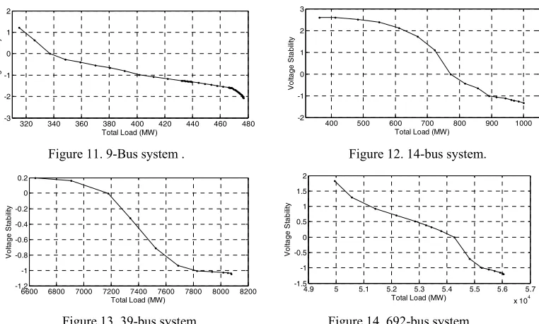
 for critically stable condition for the same contingency. Figure 11-14 depict the relation curve between the proposed voltage stability relation function  3

V

 and total load level for the four test systems, i.e. IEEE 3-machine 9-bus system, IEEE 4-machine 14-bus system, 10-machine 39-bus New England benchmark system, and a real provincial 138-machine 692-bus system respectively. From the computational results,  3

V

 decreases, monotonously and fast, with load increasing for all the systems and can well represent the voltage stability within a largest load varying range. So  3

V

 is highly recommended as the voltage stability relation function, which takes all the detailed model and dynamics of the system into consideration; and moreover the computation burden is extremely light.

     

 

2 2

3 Cr

2 Cr

V V

V

V

 



 

 (9)

To obtain the voltage stability relation function  3

V

320 340 360 380 400 420 440 460 480 -3

-2 -1 0 1 2

Total Load (MW)

V

ol

tage S

tabi

lit

y

400 500 600 700 800 900 1000

-2 -1 0 1 2 3

Total Load (MW)

V

o

lta

g

e

S

ta

b

ility

Figure 11. 9-Bus system . Figure 12. 14-bus system.

6600 6800 7000 7200 7400 7600 7800 8000 8200 -1.2

-1 -0.8 -0.6 -0.4 -0.2 0 0.2

Total Load (MW)

V

ol

tage S

tab

ility

4.9 5 5.1 5.2 5.3 5.4 5.5 5.6 x 105.74

-1.5 -1 -0.5 0 0.5 1 1.5 2

Total Load (MW)

V

ol

tag

e S

tabi

lit

y

Figure 13. 39-bus system. Figure 14. 692-bus system.

In Figure 11, the maximum load beyond which the IEEE 3-machine 9-bus system becomes unstable for the same contingency depicted in Section III is 337MW, which is smaller than both the maximum loadability 381MW after contingency and the maximum loadability 477MW before contingency according to P-V curves in Figure 4. So other three systems do.

System loadability margin produced by P-V curve is static data, determined by power system network structure and parameters, and system operating point, also closely connected with generator reactive power limitation, however system stable condition is influenced by other more detailed factors: fault severity, e.g. the fault clearing time, dynamic characteristics of synchronous machine and load, etc. Voltage stability relation function  3

V

 can express system loadability better than traditional static voltage stability indexes under contingency.

Summary

A novel voltage stability relation function based on an one-machine-infinite-bus (OMIB) equivalent is proposed in this paper. This index is stricter than traditional static voltage stability indexes and valid in a relatively large load variation range near the critical stable loading level, which will help to deal with load perturbation problems in optimal control[13-15], e.g. in solving transient stability constrained optimal power flow and transient stability excitation control optimization.

Acknowledgement

This research was financially supported by the Collaborative Innovation Center in Zhuhai (55560310) and the Fundamental Research Funds for the Central Universities (11617359).

References

[1] A. Gomez-Exposito, A.J. Conejo, and C.A. Canizares, Electric energy systems analysis and operation, New York: CRC Press. (2009) 441-456.

[4] Y. Xue, T.V. Cutsem, and M. Ribbens-Pavella, “Extended equal area criterion justification, generalizations, applications,” IEEE Transactions on. Power Systems, vol. 4, no. 1, pp. 44-52, Feb. 1989.

[5] Y. Xue, L. Wehenkel, E. Euxibie, and B. Heilbronn, “Extended equal area criterion revisited,” IEEE Transactions on. Power Systems, vol. 7, no. 3, pp. 1012-1022, Aug. 1992.

[6] Y. Zhang, P. Rousseaux, L. Wehenkel, and M. Pavella, “SIME: A comprehensive approach to fast transient stability assessment,”. in Proc. of IEE-Japan, Power and Energy’96, Osaka, Japan, 1996, pp. 1177-1182.

[7] Y. Zhang, L. Wehenkel, P. Rousseaux, and M. Pavella, “Transient stability transfer limits of a longitudinal system using the SIME method,” in Proc. of MELECON, Bari, Italy, 1996, pp. 809-815. [8] Y. Zhang, L. Wehenkel, P. Rousseaux, and M. Pavella, “SIME: A hybrid approach to fast transient stability assessment and contingency selection,” Electrical Power & Energy Systems, vol. 19, no. 3, pp. 195-208, 1997.

[9] Y. Xue and M. Pavella, “Critical cluster identification in transient stability studies,” IEE Proceedings, Part C, vol. 140, no. 6, pp. 481-489, Nov. 1993.

[10] F. Milano, “An open source power system analysis toolbox,” IEEE Transactions on. Power Systems, vol. 20, no. 3, pp. 1199-1206, Aug. 2005.

[11] IEEE Committee Report, “Excitation system models for power system stability studies,” IEEE Transactions on. Power Apparatus and Systems, vol. 100, no. 2, pp. 494-509, Feb. 1981.

[12] D. Karlsson and D.J. Hill, “Modelling and Identification of Nonlinear Dynamic Loads in Power Systems,” IEEE Transactions on Power Systems, vol. 9, no. 1, 157–166, Feb. 1994.

[13] Yulong Huang, Mingbo Liu, “Transient stability constrained optimal power flow computing by combination of trajectory sensitivity and differential evolution technique,” Power System Protection and Control, vol. 39, no. 10, pp. 18-26, May 2011 (in Chinese).

[14] Yulong Huang, Mingbo Liu, “Hybrid algorithm for solution of transient stability constrained optimal power flow,” Transactions of China Electrotechnical Society, vol. 27, no. 5, pp. 229-237, May 2012(in Chinese).