Graph Clustering: Algorithms, Analysis and Query Design

(1)

Algorithms, Analysis and Query Design

Thesis by

Ramya Korlakai Vinayak

In Partial Fulfillment of the Requirements for the degree of

Doctor of Philosophy

CALIFORNIA INSTITUTE OF TECHNOLOGY Pasadena, California

2018

(2)

Ramya Korlakai Vinayak ORCID: 0000-0003-0248-9551

(3)

(4)

ACKNOWLEDGEMENTS

First and foremost, I want to thank my advisor, Prof. Babak Hassibi, for his guid-ance and kindness. He has been a great teacher and a mentor. I thank him for giving me the opportunity to explore my research interests and help me grow as an inde-pendent researcher. I have not only learned mathematical tools from him, but also how to think about various problems and how approach them, and how to keep an eye open for useful and interesting problems. I am deeply thankful to all my the-sis committee members, Prof. Adam Wierman, Prof. Pietro Perona, Prof. Venkat Chandrasekaran, and Prof. Yisong Yue. It has been a pleasure to have them on my committee. Their guidance and feedback have immensely helped me in shaping my research ideas.

My lab mates have been great company in this journey at Caltech. I would like to thank Samet, who guided me in my first year in the lab introduced me to the problem of graph clustering. I want to thank all my lab mates – Samet, Matt, Wei, Christos, Weal, Ahn, Bose, Ehsan, Navid, Kishore, Fariborz, Ahmed, Anatoly, Philipp, and Hikmet for all the wonderful conversations whether it was research or politics or entertainment. I will dearly miss the Friday lunch group meetings. I want to thank my undergraduate mentees, Berk, Tijana, and Anna; working with them has helped me grow as a researcher. I also want to thank everyone from the Caltech Vision Group for always welcoming me to their group meetings and for all the wonderful discussions and feedback.

(5)

(Arun), Prasanna, Vinay, Akila, Adithi, Siva, Subhash, Prakash, and Samaadhi (Ar-jun) for being there not only to share the good times but also for being supportive through the tough times.

I am deeply grateful to Caltech’s International Students Program, the Caltech Y, and the Caltech Center for Diversity for all the events that made me feel welcome at Caltech and gave me the opportunity to experience and explore LA. I am thankful to Shirley, Tanya, and Katie in the EE department and Tess from registrar’s office for making my life as a student very smooth.

(6)

ABSTRACT

A wide range of applications in engineering as well as the natural and social sci-ences have datasets that are unlabeled. Clustering plays a major role in exploring structure in such unlabeled datasets. Owing to the heterogeneity in the applica-tions and the types of datasets available, there are plenty of clustering objectives and algorithms. In this thesis we focus on two such clustering problems: Graph ClusteringandCrowdsourced Clustering.

In the first part, we consider the problem of graph clustering and study convex-optimization-based clustering algorithms. Datasets are often messy – ridden with noise, outliers (items that do not belong to any clusters), and missing data. There-fore, we are interested in algorithms that are robust to such discrepancies. We present and analyze convex-optimization-based clustering algorithms which aim to recover the low-rank matrix that encodes the underlying cluster structure for two clustering objectives:clustering partially observed graphsandclustering similarity matrices with outliers. Using block models as generative models, we characterize the performance of these convex clustering algorithms. In particular, we provide

explicit bounds, without any large unknown constants, on the problem parameters that determine the success and failure of these convex approaches.

(7)

(8)

PUBLISHED CONTENT AND CONTRIBUTIONS

[VH16a] Ramya Korlakai Vinayak and Babak Hassibi. “Crowdsourced Clus-tering: Querying Edges vs Triangles”. In:Advances in Neural Infor-mation Processing Systems. 2016, pp. 1316–1324. url: http : / /

papers . nips . cc / paper / 6499 crowdsourced clustering -querying-edges-vs-triangles.pdf.

Ramya Korlakai Vinayak is the lead author and main contributor to the above paper.

[VH16b] Ramya Korlakai Vinayak and Babak Hassibi. “Similarity clustering in the presence of outliers: Exact recovery via convex program”. In:

IEEE International Symposium on Information Theory (ISIT). 2016, pp. 91–95. url: http : / / ieeexplore . ieee . org / abstract /

document/7541267/.

[VOH14a] Ramya Korlakai Vinayak, Samet Oymak, and Babak Hassibi. “Graph clustering with missing data: Convex algorithms and analysis”. In: Ad-vances in Neural Information Processing Systems. 2014, pp. 2996– 3004. url: http : / / papers . nips . cc / paper / 5309 graph

-clustering- with- missing- data- convex- algorithms- and-analysis.pdf.

[VOH14b] Ramya Korlakai Vinayak, Samet Oymak, and Babak Hassibi. “Sharp performance bounds for graph clustering via convex optimization”. In:

IEEE International Conference on Acoustics Speech and Signal Pro-cessing (ICASSP). 2014, pp. 8297–8301.url:http://ieeexplore.

ieee.org/abstract/document/6855219/.

[VZH17] Ramya Korlakai Vinayak, Tijana Zrnic, and Babak Hassibi. “Tensor-based Crowdsourced Clustering via Triangle Queries”. In: IEEE In-ternational Conference on Acoustics Speech and Signal Processing (ICASSP). 2017.url:http://ieeexplore.ieee.org/abstract/

document/7952571/.

(9)

LIST OF ILLUSTRATIONS

Number Page

1.1 Visualization of an example social network. . . 3

1.2 Visualization of an example protein-protein interaction network . . . 3

1.3 [A toy example for graph clustering. . . 5

1.4 Example of an edge query: “Do these two birds belong to the same species?” . . . 10

1.5 Example of a triangle query: “Which of these birds belong to the same species?” . . . 10

1.6 Configurations for a triangle query. . . 11

2.1 [A toy example for graph clustering. . . 14

2.2 Depiction of exact recovery guarantee for Simple Program . . . 21

2.3 Region of success (white region) and failure (black region) of Pro-gram 2.1.4 with λ= 1.01D−_min1 . The solid red curve is the threshold for success (λ <Λsucc) and the dashed green line which is the thresh-old for failure (λ >Λfail) as predicted by Theorem 1. . . 26

2.4 Region of success (white region) and failure (black region) of Pro-gram 2.1.4 with λ= 1.01D−_min1 . The solid red curve is the threshold for success (λ <Λsucc) and the dashed green line which is the thresh-old for failure (λ >Λfail) as predicted by Theorem 1. . . 27

2.5 Region of success (white region) and failure (black region) of Pro-gram 2.1.7 with λ = 0.49 ˜Λsucc. The solid red curve is the threshold for success (D˜min> lambda−1) as predicted by Theorem 2. . . 28

2.6 Comparison range of edge probability p for Simple Program 2.1.4 and Improved Program 2.1.7. . . 28

2.7 Result of using (a) Program 2.1.4 (Simple) and (b) Program 2.1.7 (Improved) on the real data set. . . 30

2.8 Comparing the clustering output after running Program 2.1.4 and Program 2.1.7 with the output of applying k-means clustering di-rectly onA(with unknown entries set to 0). . . 30

(12)

2.10 Sample images of three breeds of dogs that were used in the MTurk

experiment. . . 33 2.11 Illustration of{Ri,j}dividing[n]×[n]into disjoint regions similar

to a grid . . . 35 3.1 Fraction of correct entries in the solution obtained by running

Pro-gram 3.1.1 withn = 100, similarity between the clusters:µout = 0.2,

standard deviation of noise:σ = 0.1and varying similarity inside the

clustersµin, for the three cases: (1) no outliers, (2) small number of

outliers and (3) large number of outliers. Solid blue line is the curve

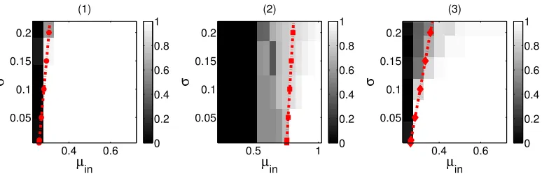
from the simulations and the dashed green line is the threshold for µinpredicted by theory. . . 48 3.2 Region of success (white) and failure (black) for Program 3.1.1 on

synthetic data of n = 600, µout = 0.20, for varying µin and σwith (1)3clusters size200each (no outliers),λ= 1.001Λ, (2)2clusters

of size 200 and rest nout = 200 outliers, λ = 1.001(Λ +µoutnout)

(recover only the clusters), (3)2clusters of size200and restnout =

200 outliers, λ = 1.001Λ(recover outliers as a cluster). The dotted

red lines are the thresholds for µin predicted by the theory for the

correspondingσ. . . 50 3.3 Rounded output after running Program 3.1.1 on real datasets. (1) Iris

and (2)digit1000. . . 52 3.4 Sorted eigenvalues for the rounded output X and the normalized

Laplacian of the similarity matrixAfor Iris anddigit1000datasets. 52 4.1 Example of an edge query: “Do these two birds belong to the same

species?” . . . 54 4.2 Example of a triangle query: “Which of these birds belong to the

same species?” . . . 54 4.3 Configurations for a triangle query that are (a) observed and (b) not

allowed. . . 55 4.4 Fraction of entries in error in the matrix recovered via Program 4.4.1. 61

4.5 VI for Spectral Clustering output for varying edge density inside the clusters. 64

4.6 VI for Spectral Clustering output for varying number of clusters (K). . . 64

5.1 Example of a triangle query. . . 69 5.2 Configurations for a triangle query that are (a) observed and (b) not

(13)

5.3 Comparison of VI (averaged over 10 experiments) for clustering

us-ing the tensor (filled usus-ing different encoding schemes) compared to

that obtained using adjacency matrix, for varying different

parame-ters for the Conditional Block Model (Section 5.4.3). . . 75 5.4 Comparison of VI (averaged over 10 experiments) for clustering

us-ing the tensor (filled usus-ing different encoding schemes) compared to

that obtained using adjacency matrix, for varying different

parame-ters for the Triangle Block Model (Section 5.4.3) . . . 76 6.1 Comparison of the upper bounds on the total number of queries

re-quired for exact clustering by active and random querying for large

clusters (sizeΘ(n)). . . 89 6.2 Comparison of the upper bounds on the total number of queries

re-quired for exact clustering by active and random querying for small clusters (sizeΘ(√n)) . . . 89 6.3 Empirical pdf ofTij . . . 90 6.4 Minimum, maximum, median, mean (along with standard deviation)

of the number of repeated queries as a function of varying error

prob-ability (p). Averaged over10trials). . . 91 6.5 Minimum, maximum, median, mean (along with standard deviation)

of the number of repeated queries as a function of varying number of clusters (K). Averaged over10trials. . . 91 6.6 Minimum, maximum, median, mean (along with standard deviation)

of the number of repeated queries as a function of varying number of

items (n). Averaged over10trials. . . 92 6.7 Cumulative averages of the answers given by crowdworkers for

re-peated queries for 6sample items. The first row corresponds to the

experiment where Query(i,j) is repeated with samejand the second

row corresponds to the experiment wherej is chosen randomly from cluster(j) each time. Note that the true answer is at the top of each

plot. . . 94 A.1 Illustration of{Ri,j}dividing[n]×[n]into disjoint regions similar

(14)

LIST OF TABLES

Number Page

2.1 Empirical Parameters from the real data. . . 32 2.2 Number of miss-classified images . . . 32 3.1 Percentage of mis-classified data points . . . 51 4.1 Query confusion matrix for the triangle block model for the

homo-geneous case. . . 58 4.2 Query confusion matrix for the conditional block model for the

ho-mogeneous case. . . 59 4.3 Summary of the data colleced in the real experiments. . . 65 4.4 VI for clustering output by k-means and spectral clustering for the

Dogs3 dataset. . . 65 4.5 VI for clustering output by k-means and spectral clustering for the

Birds5 dataset. . . 65 6.1 Various statistics for the number of repeated queries, the total

num-ber of queries made and the percentage of node pairs in error after

(15)

C h a p t e r 1

INTRODUCTION

Unsupervised learning plays a crucial role in finding patterns and extracting useful information from unlabeled data. Clustering is the most widely used unsupervised learning tool. Many applications have data that is unlabeled, for example, biolog-ical images, data from observational astronomy, images, videos and texts on the internet, and so on. Clustering broadly refers to grouping together data items that are similar.

Clustering is in general an ill-posed problem and is meaningful when defined more concretely for a given objective. There are two main aspects to clustering. The first aspect concerns with the representation of data, the definitions of similarity and clusters, and the evaluation metrics. As the applications and the types of data avail-able differ widely, so do the representations of data and definitions of similarity and clusters. The second aspect deals with algorithms for clustering a dataset, given an objective. This thesis looks at the second aspect in the context ofgraph clustering

andcrowdsourced clustering.

Clustering or cluster analysis originated in the1930’s with the work of Driver and Kroeber [DK32] in anthropology to understand the similarities between different cultural tribes in the Americas and was further used in psychology [Zub38;Try39] for personality analysis. Today clustering is an essential tool for quantitative anal-ysis in many applications in engineering, the natural and social sciences. Given its applications in various areas, different point of views and many algorithms have been proposed. Hierarchical clustering, center based clustering, density based clus-tering, data partitioning, mixture models, etc., are some of the examples of different view points for clustering. There are many clustering algorithms, like means, k-median, linkage based agglomorative algorithms, partition based algorithms, spec-tral clustering, expectation-maximization, and variational inference based maxi-mum likelihood algorithms, message passing algorithms, Monte Carlo methods, and many more. Given the breadth of research in clustering, an in-depth survey of the subject is out of the scope of this thesis. We refer the readers to the surveys and books dedicated to clustering [JMF99;VB05;AR13;XT15].

(16)

non-expert humans to solve problems that are difficult to solve by machines. Us-ing crowdsourcUs-ing to collect labeled data became popular around mid-2000’s with games with a purpose [Von06] and recaptcha [Von+08]. Today crowdsourcing is used for a wide variety of tasks including collecting data [Ray+10], surveys [Beh+11], and tasks like translation, summarization, transliteration [Sno+08;SBS12;Kha+14], and many more. There are several platforms such as Amazon Mechanical Turk and Crowdflower available that bring the requesters (those who want the tasks done) and workers (those who are willing to do the tasks for monetary compensation or voluntarily) together. Many times enthusiastic general public voluntarily contribute to scientific discoveries via platforms like Zooinverse, Planet Hunters, etc. Applica-tions of crowdsourcing for academic endeavors range from creating labeled datasets for training and testing supervised machine learning algorithms [Ray+10;Sno+08;

Von+08;SF08;Wel+10;Yi+12] to making scientific discoveries [SPD14;Lin+13]. In this thesis, we focus on using crowdsourcing for clustering.

In the rest of this chapter we discuss the motivation and relevant literature, and summarize the contributions made in this thesis for problems in graph clustering and crowdsourced clustering.

1.1 Graph Clustering

(17)

[image:17.612.168.445.102.366.2]

Figure 1.1: Visualization of a social network around an individual [urla].

[image:17.612.169.444.454.656.2]

(18)

Different versions of this problem have been studied as graph clustering [Sch07;

FTT04; CGW05], correlation clustering [EF03; BBC04; GG06], graph

partition-ing on planted partition model [CK01;McS01], community detection [FH16], etc. Many graph clustering objectives are NP-hard in the worst case. However, real world datasets are more structured and it is frequently observed that simple cluster-ing algorithms perform quite well in practice. A natural question that arises is:

what are the structural properties of datasets that enable computationally efficient clustering?

The pertinent questions are: (1) How much should the difference between the edge density (or similarity) between the nodes inside a cluster and the edge density (or similarity) between the nodes from different clusters be? (2) When can we be con-fident that this difference is due to underlying structure in the data and not out of randomness or due to noise?

In order to understand these fundamental bottlenecks, we study simple generative

block modelswhich assume different distribution of edges (or similarity) inside the clusters and between the clusters. For example, consider the case of an unweighted graph with disjoint clusters. A popular block model in this setting is theStochastic Block Model(SBM) or the planted partition model [HLL83;CK01] which assumes that given the assignment of nodes in a graph to (disjoint) clusters, each pair of nodesiandj is connected independently with probabilitypif they are in the same cluster and with probability q otherwise. Using the Stochastic Block Model, our analysis of simple convex programs for graph clustering (based on low-rank plus sparse decomposition of the adjacency matrix) shows that clusters that are small and sparse are the bottlenecks.

A common and well justified criticism of such block models is that they are not realistic. While the block models are simplistic, they capture the essence of the problem without getting lost in too many details. Studying these simple models can provide valuable insights into the fundamental bottlenecks for clustering. As statistician George Box famously said [B+87]:

(19)

[image:19.612.115.495.82.232.2]

(a) Toy example. (b) Ideal clusters.

Figure 1.3: A toy example for a graph clustering with clusters (a) and the corre-sponding ideal cluster structure (b).

Convex Programs for Clustering

Real world datasets are messy. They are noisy, have missing data and contain out-liers – nodes that do not belong to any clusters. We need clustering algorithms to be robust to such discrepancies. We also want the algorithms to be tractable and com-putationally efficient. Further, we want these algorithms to be amenable to analysis that help us understand their strengths and weaknesses and provide guarantees as to when they can successfully recover the clusters.

Suppose a given graph has clusters. For example, consider the graph in Figure1.3a, which has the following adjacency matrix:

                  

1 1 1 0 1 0 0 0 0 0 0 0 0 0

1 1 1 1 1 0 0 0 0 0 0 0 0 0

1 1 1 0 1 0 1 0 0 0 1 0 0 0

0 1 0 1 0 0 0 0 0 0 0 0 0 0

1 1 1 0 1 0 0 0 0 0 0 0 0 0

0 0 0 0 0 1 1 0 1 1 0 0 0 0

0 0 1 0 0 1 1 1 1 0 0 0 0 0

0 0 0 0 0 0 1 1 1 0 0 0 0 0

0 0 0 0 0 1 1 1 1 0 0 0 0 0

0 0 0 0 0 1 0 0 0 1 0 0 0 0

0 0 1 0 0 0 0 0 0 0 1 1 1 0

0 0 0 0 0 0 0 0 0 0 1 1 1 1

0 0 0 0 0 0 0 0 0 0 0 1 1 1

                   .

(20)

cluster structure that is a union of disjoint cliques (see Figure1.3b):                   

1 1 1 1 1 0 0 0 0 0 0 0 0 0

0 0 0 0 0 1 1 1 1 1 0 0 0 0

0 0 0 0 0 0 0 0 0 0 1 1 1 1

                   ,

(note that the rank of this matrix is3which is equal to the number of clusters in this example) plus noise that captures the missing edges inside the cliques and the extra edges that go between the cliques. Note that the adjacency matrix corresponding to a union of disjoint cliques (Figure1.3b) has rank equal to the number of clusters (we assume that the diagonal of the adjacency matrix is all 1’s). In many applications the number of clusters is much smaller than the number of nodes in the graph, and hence the ideal clustered graph has a low-rank adjacency matrix. Our aim is to recover the low-rank matrix corresponding to the union of disjoint cliques since it is equivalent to finding the clusters.

Several graph clustering objectives can be posed as low-rank matrix recovery and completion problems. Developments in convex optimization techniques to recover low-rank matrices [CR09;Can+11;CPW10;Cha+11] via nuclear norm1 minimiza-tion has recently led to the development of several convex algorithms to recover clusters in a graph [XCS10;AV14;AV11;Che+14;OH11;CSX12;Ame13]. This

convex approach is robust to noise, outliers, missing data and unbalanced clusters. Moreover, these convex approaches are often semi-definite programs (SDPs) that have polynomial computational complexity.

We consider convex algorithms for two clustering objectives. The first objective we consider is the problem of finding clusters in an unweighted graph when only partial observations are available. The second is the problem of clustering a similarity matrix or, equivalently, a weighted graph in the presence of outliers. Chapter2and Chapter3of this thesis are devoted to these two objectives.

(21)

Graph Clustering with Missing Data

Clearly, a graph onnnodes has n₂possible edges. In many practical scenarios, it is too expensive to measure or infer the existence or non-existence of each of these edges. Thus the problem of finding clusters in a graph that ispartially observedor hasmissing datais of interest.

Our goal is to understand the fundamental trade-offs of this problem. In particular, we are interested in exploring the following questions:

1. How much noise can be tolerated? In particular, how much should the sepa-ration between the density of edges inside and between the clusters be? 2. How many observations are required to guarantee the exact recovery of

clus-ters?

3. How large should the clusters be relative to the size of the graph for them to recovered exactly? How much does the balanced or unbalancedness of the relative cluster sizes matter?

4. How does the presence of outliers affect the ability to recover the clusters?

We consider two convex programs based on low-rank plus sparse decomposition of the observed adjacency matrix. We analyze their performances using the popular

Stochastic Block Model where the edges in the graph are independent and (in the simplest case) exist with probabilitypinside the clusters andqbetween the clusters. To incorporate missing data, we further assume that each edge is independently observed with probabilityr. We show that the clusters that are both small and sparse are the bottlenecks. In simple terms, we show the following sufficient condition for exact recovery of clusters:

nmin ≥2σ

√

n

√

r(p−q),

where nmin is the size of the smallest cluster and σ captures the noise due to the

missing edges inside the cliques and the extra edges that go between the cliques.

When√r(p−q) = Θ(1), our result shows that the sufficient condition for exact

re-covery requires the minimum cluster size to be at leastΩ(√n)which improves the previously known bound ofΩ(pn(logn)4₎_{. Unlike previous results on convex}

(22)

results do not involve unknown large constants. Furthermore, our analysis also pro-vides precise conditions under which the convex approach fails in exact recovery, thus advancing the understanding of thephase transitionfrom failure to success for the convex approach. Apart from providing theoretical guarantees for the problem considered and corroborating them with simulations, we also apply the convex pro-gram to a real data set obtained by crowdsourcing an image labeling task. Chapter2 presents details of the problem of graph clustering with missing data and is based on the following papers [VOH14b;VOH14a].

Similarity Clustering in the Presence of Outliers

Several datasets have heterogeneous attributes, e.g. in census data, each individual person has attributes such as age and income which are numerical and race, reli-gion, address etc., that are categorical. Depending on the application domain, it is often possible to construct a similarity map that assigns a numerical value to how similar two data items are, using which we can construct asimilarity matrix. Such similarity matrices are generalynoisybecause of the inherent noise in the data itself and the imperfections in the similarity maps. The data might also containoutliers, that is, data points that do not belong to any cluster.

We consider a convex program that aims to recover a (low-rank) matrix that reflects the true cluster structure from the noisy similarity matrix with outliers and no other side information. We analyze the convex program for a generative block model and provideprecise thresholds(not orderwise) as a function of the problem parameters for successfully recovering the clusters. In simple terms we show the following sufficient condition for exact recovery of clusters:

nmin ≥

2√n σ+ 1

µin−µout ,

whereµin andµout are the average similarities inside and between the clusters re-spectively andσis the standard deviation of the noise in the similarity matrix. Al-though our analysis uses the problem parameters, the program itself does not need to know them.

In the case of unweighted graphs,l1 penalty on the noise is a natural loss function

and as an added bonus thel1 penalty is also robust to outliers. However, for

similar-ity matrices (or weighted graphs) thel1penalty does not fit the noise characteristics.

(23)

is not inherently robust to outliers, we need to understand how the presence of out-liers affect the recovery of clusters. We show that, in the presence of a large number of outliers (≥ Ω(√n)), the convex program forces the outliers to form their own cluster without disturbing the structure of the rest of the clusters.

Our analysis provides a complete picture of the fundamental bottlenecks of the sim-ple convex program for similarity clustering. In contrast to the previously known results in this area [Ame14], our results do not involve large unknown constants and provides insights into the behavior of the solution in the presence of large number of outliers as well as the effect of noise variance. We corroborate our theoretical guar-antees with extensive numerical simulations as well as evaluate the performance of the convex program on real datasets. Details on this problem are presented in Chapter3and are based on the following paper [VH16b].

1.2 Crowdsourced Clustering

(24)

[image:24.612.150.459.79.194.2]

Figure 1.4: Example of an edge query: “Do these two birds belong to the same species?”

Triangle vs. Edge Querying

In any crowdsourcing system, we expect noisy answers from the crowd workers. Noise in the responses from crowd workers is not solely due to their lack of ex-pertize or ability. Design of queries has a significant impact on the noise levels in the responses by the crowd workers. In Chapter4 we consider the problem of crowdsourced clustering using similarity queries and compare two types of queries: (1) random edge queries, where a pair of images is revealed for comparison (Fig-ure1.4), and (2) random triangle queries, where a triplet is revealed (Figure1.5). Using intuitive generative models, we show that the average number of errors in the entries of the adjacency matrix decreases when it is filled via triangle queries

[image:24.612.127.489.491.669.2]

(25)

1"

2"

3"

lll

!

1"

2"

3"

llm

!

1"

2"

3"

lml

!

1"

2"

3"

mll

!

1"

2"

3"

lmj

!

1"

2"

3"

1"

2"

3"

1"

2"

3"

(a)"Allowed"

(b)"Not"allowed"

Figure 1.6: Configurations for a triangle query.

compared to when it is filled using using edge queries. Empirical evidence, based on extensive simulations, as well as experiments on Amazon Mechanical Turk us-ing two real data sets, strongly suggests that, for a fixed query budget (the cost of a query is set proportional to the average response time of the workers), triangle queries significantly outperform edge queries. In particular, under a fixed budget, triangle queries double the number of observed entries of the adjacency matrix

while decreasing the average number of errorsby5%.

For reliably clustering the noisy and partially observed data, we leverage the con-vex algorithms and analysis from our study of graph clustering. Our analysis of the graph clustering problem (recall the discussion in Section 1.1 and for details see Chapter 2) provides us the insight that convex clustering algorithms perform well when there is a good separation between the edge density inside and between clusters and when we make enough observations. Since triangle queries reduce the noise and provide more data, we expect graph clustering algorithms to work better on the adjacency matrices filled using triangle queries. However, the analysis in Chapter2assumes that the entries of the adjacency matrix are independent, which does not hold when it is filled via triangle queries. We extend the analysis to provide theoretical guarantee for the exact recovery of clusters via random triangle queries. Chapter4has more details and is based on the following paper [VH16a]).

Tensor Embedding for Triangle Queries

In Chapter4, we demonstrate that using triangle queries to fill the adjacency matrix gives better clustering results than using edge queries. However, it does not exploit the fact that the response to a triangle query is associated with a triplet and a natural question that arises at this point is whether exploiting this fact adds any benefit. We explore this question in Chapter5.

(26)

clusters. In contrast, there are 5 possible answers to a triangle query (Figure1.6) and in general we need 5 symbols to represent them. We can then embed the responses to the triangle queries into a 3-rd order tensor. Surprisingly, any arbitrary choice of symbols will generally not lead to a true tensor with rank equal to the number of clusters. We propose a general encoding scheme and provide sufficient condi-tions on it to give a true tensor with unique low-rank CP-decomposition with rank equal to the number of clusters. We also provide extensive numerical simulations that show that using tensor decomposition methods can improve over clustering ob-tained via the adjacency matrix. Details are available in Chapter5(which is based the following paper [VZH17]).

Active Querying for Crowdsourced Clustering

Querying for similarity between random pairs or triples of items followed by per-forming clustering on the adjacency matrix filled using these queries provides rea-sonable clusters. However, the bottlenecks in terms of how many observations are needed and what is the size of the smallest cluster that can be recovered are dic-tated by the graph clustering step. A natural question that arises is whether we can escape these bottlenecks as we are using crowdsourcing. We explore this question in Chapter 6and consider an active querying setting for crowdsourced clustering. We propose a novel algorithm which uses confidence intervals that shrink as more queries are made and is based on the law of the iterated logarithm [Jam+14]. The algorithm we propose can reliably find the clusters without the knowledge of any parameters and without the small cluster barrier posed by graph clustering. In par-ticular, under mild assumptions, we show that the number of queries made by the proposed algorithm is upper bounded by,

O

nK

∆2 log

nlog 1 ∆

,

where∆ := min{p−1 2,

1

2 −q}.In contrast with the state-of-the-art algorithms for

(27)

C h a p t e r 2

GRAPH CLUSTERING WITH MISSING DATA

In this chapter, we consider the problem of finding clusters in an unweighted graph when the graph is partially observed. We analyze two programs that are based on the convex optimization approach for low-rank matrix recovery using nuclear norm minimization withl1-norm penalty on the noise. For the commonly used Stochastic

Block Model, we obtain explicit bounds (not orderwise) on the parameters of the problem (size and sparsity of clusters, the amount of observed data) and the regular-ization parameter that characterize the success and failure of the convex programs. We corroborate our theoretical findings through extensive simulations. We also run our algorithm on a real data set obtained from crowd sourcing an image clus-tering task on the Amazon Mechanical Turk, and observe significant performance improvement over traditional clustering methods such as k-means and spectral clus-tering. This chapter is based on our papers [VOH14b;VOH14a].

2.1 Introduction

Clustering [JMF99] broadly refers to the problem of identifying data points that are similar to each other. It has applications in various problems in machine learning, data mining [EKX95;XJK99], social networks [Mis+07;DR01;For10], bioinfor-matics [XOX02; YL05], etc. In many applications, data has a graphical structure. For example, in social network, individuals are the nodes in the graph and the edges represent friendship between the nodes. Another example is a protein-protein inter-action network, where the nodes in the graph are proteins and an edge between two proteins represents biochemical or electrostatic interaction between them. Given an

(28)

know whether there exists an edge between them or not, whereas for the rest of the node pairs we do not have this knowledge. Given a graph with partial observations, we still want to identify the underlying clusters. This leads us to the problem of clustering graphs withmissing data.

In this chapter, we consider the problem of identifying clusters when the input is a partially observed adjacency matrix of an unweighted graph and look at two convex algorithms in this regard. We use the popular Stochastic Block Model

(SBM) [HLL83], also called as Planted Partition Model [CK01], to analyze the performance of these convex algorithms. SBM is a random graph model where the edge probability depends on whether the pair of nodes being considered belong to the same cluster or not. More specifically, the edge probability is higher when both nodes belong to the same cluster. Further, we assume that each entry of the adja-cency matrix of the graph is observed independently with probability r. We will define the model in detail in Section2.2.

2.1.1 Clustering by Low-Rank Matrix Recovery and Completion

The idea of using convex optimization for clustering has been proposed in [XCS10;

Che+14; AV14; AV11; OH11; CSX12; Che+14]. While each of these works

dif-fer in certain ways, and we will comment on their relation to the current paper in Section 2.1.3, the common approach they use for clustering is inspired by recent works on low-rank matrix recovery and completion via regularized nuclear norm (trace norm) minimization [CR06;CR09;Can+11;CPW10;Cha+11].

In the case of unweighted graphs, an ideal clustered graph is a union of disjoint

[image:28.612.112.497.524.672.2]

(a) Toy example. (b) Ideal clusters.

(29)

cliques (Figure 2.1b). Given the adjacency matrix of an unweighted graph with clusters – denser connectivity inside the clusters compared to outside (Figure2.1a), we can interpret it as an ideal clustered graph with some missing edges inside the clusters and some erroneous edges in between the clusters. Recovering the low-rank matrix corresponding to the disjoint cliques is equivalent to finding the clusters. Ideally we want to solve the following optimization problem:

minimize

L,S rank(L) +λkSk0 (2.1.1) subject to

Li,j ∈ {0,1}, (2.1.2)

Lobs+Sobs =Aobs, (2.1.3)

where rank(Y)is the rank of the matrixY, kYk0 is thel0-norm ofY (number of

non-zero entries in the matrixY), Lobs andSobs are the low-rank and sparse parse matrices respectively over the observed entries of A, and λ ≥ 0 is the regular-ization parameter that balances the weight between rank(L)andkSk0. The above

optimization problem (Program2.1.1) is NP-hard. Both the terms in the loss func-tion, rank(.) and l0-norm, are non-convex functions. Furthermore, the constraint

on the entries of L (Equation 2.1.2) is a very difficult set to optimize over. We note that the objective is a low-rank matrix recovery and completion problem with sparse corruption. This problem can be relaxed to a tractableconvex program. We consider the following convex program which aims to recover and complete the low-rank matrix (L) from the partially observed adjacency matrix (Aobs):

Simple Convex Program:

minimize

L,S kLk?+λkSk1 (2.1.4)

subject to

1≥Li,j ≥0 for alli, j ∈ {1,2, . . . n} (2.1.5)

Lobs+Sobs =Aobs, (2.1.6)

where λ ≥ 0 is the regularization parameter, k.k? is the nuclear norm (sum of the singular values of the matrix), and k.k1 is thel1-norm (sum of absolute values

(30)

Program2.1.4is very simple and intuitive. Further, it does not require any informa-tion other than the observed part of the adjacency matrix. In [Che+14], the authors analyze Program2.1.4without the constraint (2.1.5). While dropping (2.1.5) makes the convex program less effective, it does allow [Che+14] to make use of low-rank matrix completion results for its analysis. In [OH11] and [VOH14b], the authors analyze Program2.1.4when the entire adjacency matrix is observed. In [CSX12], the authors study a slightly more general program, where the regularization param-eter is different for the extra edges and the missing edges. However, the adjacency matrix is completely observed.

It is not difficult to see that, when the edge probability inside the clusters isp < 1₂, (as n → ∞) Program 2.1.4 will return L0 _{= 0} _{as the optimal solution (since if}

the cluster is not dense enough it is more costly to complete the missing edges). As a result our analysis of Program2.1.4, and the main result of Theorem1 (Sec-tion2.3.1), assumesp >1/2. Clearly, there are many instances of graphs we would like to cluster where p < 1/2. If the total size of the cluster region (i.e, the total number of edges in the cluster, denoted by|R|) is known, then the following con-vex program can be used, and can be shown to work forp <12(see Theorem2in Section2.3.2).

Improved Convex Program:

minimize

L,S kLk?+λkSk1 (2.1.7)

subject to

1≥Li,j ≥Si,j ≥0 for alli, j ∈ {1,2, . . . n} (2.1.8)

Li,j =Si,j wheneverAobsi,j = 0 (2.1.9)

sum(L)≥ |R|. (2.1.10)

As before,Lis the low-rank matrix corresponding to the ideal cluster structure and λ ≥ 0is the regularization parameter. However,S is now the sparse error matrix that accounts only for the missing edges inside the clusters on the observed part of adjacency matrix. [OH11] and [Ame13] study programs similar to Program2.1.7 for the case of a completely observed adjacency matrix. In [Ame13], the con-straint2.1.10is a strict equality. In [AV11] the authors analyze a program close to Program2.1.7but without thel1penalty.

(31)

suggest that the solution is not very sensitive to the choice ofR.

2.1.2 Our Contributions

Our contributions are multifold:

1. We analyze the Simple Convex Program2.1.4 for the SBM with partial ob-servations. We provide explicit bounds on the regularization parameter as a function of the parameters of the SBM, that characterizes the success and failure conditions of Program 2.1.4(see results in Section 2.3.1). We show that clusters that are either too small or too sparse constitute the bottleneck. Our analysis is helpful in understanding thephase transitionfrom failure to success for the simple approach.

2. We also analyze the Improved Convex Program 2.1.7. We explicitly char-acterize the conditions on the parameters of the SBM and the regularization parameter for successfully recovering clusters using this approach (see results in Section2.3.2).

3. Apart from providing theoretical guarantees and corroborating them with simulation results (Section 2.4), we also apply Programs 2.1.4and 2.1.7on a real data set (Section2.4.3) obtained by crowdsourcing an image labeling task on Amazon Mechanical Turk.

2.1.3 Related Work

In [Che+14], the authors consider the problem of identifying clusters from partially observed unweighted graphs. For the SBM with partial observations, they analyze Program 2.1.4without constraint (2.1.5), and show that under certain conditions, the minimum cluster size must be at leastO(pn(log(n))4_/r₎_{for successful}

recov-ery of the clusters. Unlike our analysis, the exact requirement on the cluster size is not known (since the constant of proportionality is not known). Also they do not provide conditions under which the approach fails to identify the clusters. Finding the explicit bounds on the constant of proportionality is critical to understanding the phase transition from failure to successfully identifying clusters.

In [AV14; AV11; OH11; CSX12; Ame13], analyze convex programs similar to

(32)

conditions for failure, and except for [OH11] they do not address the case when the data is missing.

In contrast, we consider the problem of clustering with missing data. We explic-itly characterize the constants by providing bounds on the model parameters that decide if Programs2.1.4and2.1.7can successfully identify clusters. Furthermore, for Program 2.1.4, we also explicitly characterize the conditions under which the program fails.

In [OH11], the authors extend their results to partial observations by scaling the edge probabilities byr(observation probability), which willnotwork forr < 1/2

or1/2< p <1/2rin Program2.1.4. We first analyzed Program2.1.4for the SBM and provided conditions for success and failure of the program when the entire adjacency matrix is observed [VOH14b]. In this chapter, we start with the partially observed case [VOH14a] and recover the results for the fully observed case as a special case. The dependence on the number of observed entries emerges non-trivially in our analysis.

2.2 Generative Model for Partially Observed Graphs

In this section we describe the model we consider for the partially observed un-weighted graphs with clusters which builds on the popular Stochastic Block Model (SBM) [HLL83] or the planted partition model [CK01]. Definition of SBM is given below:

Definition 2.2.1(Stochastic Block Model). LetA = AT be the adjacency matrix of a graph onnnodes withKdisjoint clusters of sizeni each,i= 1,2,· · · , K. Let

1≥ pi ≥ 0, i = 1,· · · , K and1≥ q ≥0. For1≤ l < m≤n, edge between the

nodeslandmexists independently and,

1. iflandmare in the same clusteri, then

Al,m =  



1with probability pi,

0with probability 1−pi.

2. iflandmare not in the same cluster, then

Al,m=   

1with probability q,

(33)

Ifpi > qfor eachi, then the average density of edges is higher inside the clusters compared to outside.

To capture partial observations, on top of the SBM, we assume that each edge is independently observed with probability r. We say the random variable Y has a

Φ(r, δ)distribution, for0≤δ, r ≤1, written asY ∼Φ(r, δ), if

Y =

        

1, w.p. rδ

0, w.p. r(1−δ)

∗, w.p. (1−r),

where ∗ denotes unknown. A formal definitio of the partial observation model considered in this chapter is as follows:

Definition 2.2.2 (Partial Observation Model). Let A be the adjacency matrix of a random graph generated according to the Stochastic Block Model of

Defini-tion 2.2.1. Let 0 < r ≤ 1. Each entry of the adjacency matrix A is observed independently with probabilityr. Let Aobs _{denote the observed adjacency matrix.}

Then forl > m: (Aobs₎

l,m∼Φ(r, pi)if both the nodeslandmbelong to the same

clusteri. Otherwise,(Aobs₎

l,m∼Φ(r, q).

Note that the model described can handle outliers(nodes that do not belong any clusters). So,PK

i=1ni ≤n.

2.3 Exact Recovery Guarantees

In this section we present the exact recovery guarantees for the convex programs (Program2.1.4and Program2.1.7). Before we state the results formally, we need some notations. We deonte the set{1,2,· · · , n}by [n]. Let the union of regions induced by the clusters be denoted byRand its complementRc _{= [}_n_]_×_[_n_]_{− R}_. Note that |R| = PK

i=1n 2

i and |Rc| = n2 −

PK

i=1n 2

i. Let the minimum edge density inside the clusters bepmin := min

1≤i≤Kpi, the minimum cluster size benmin:=

min

1≤i≤Kni, and the maximum cluster size benmax:= max1≤i≤Kni.

We note that, in this chapter, when we say a convex programsucceeds, we mean that itexactlyrecovers the adjacency matrix corresponding to the underlying cluster structure, that is, the matrixL0_{, such that,}

L0_lm =

  

1, iflandmare in the same cluster, and

(34)

2.3.1 Simple Convex Program

Recall the Simple Convex Program (Program2.1.4): minimize

L,S kLk?+λkSk1 subject to

1≥Li,j ≥0 for alli, j ∈[n]

Lobs+Sobs =Aobs.

In a nutshell, our analysis shows that

the clusters that are both small and sparse are the bottlenecks.

The quantity that determines whether Program2.1.4can recover a cluster exactly is itseffective densitywhich captures both its the size and sparsity, defined as

Di :=nir(2pi −1).

Let the smallest effective density be, Dmin = min

1≤i≤KDi. There are two thresholds on the minimum effective density that determine the conditions for succeess and failure of Program2.1.4. The threshold for success is defined as follows,

Λ−_succ1 := 2r√n r

1

r −1 + 4q(1−q)

+ max

1≤i≤K2r

√

ni r

2(1

r −1) + 4 (q(1−q) +pi(1−pi)).

Threshold for failure is defined as follows:

Λ−_fail1 :=

v u u

trq 1−

K X

i=1

n_i

n

2

! n.

We note that the thresholds,ΛsuccandΛfaildepend only the parameters of the model

and simple algebra shows thatΛ−_fail1 <Λ−1

succ.

For random graphs generated according to the Partial Observation Model of Def-inition (2.2.2) with K disjoint clusters of sizes {ni}Ki=1, and probabilities {pi}Ki=1

andq, such thatpmin > 1₂ > q >0, the following theorem provides exact recovery guarantees for Program2.1.4.

Theorem 1(Simple Program). WheneverDmin >Λ−succ1 , for any λ∈ D −1

min, Λsucc

,

(35)

𝑬𝑫𝒎𝒊𝒏

1 Ʌ𝒔𝒖𝒄𝒄

1 Ʌ𝒇𝒂𝒊𝒍

Gap Success

Failure

(a) Feasibility of Program2.1.4in terms of the minimum effective density (Dmin).

Ʌ𝒇𝒂𝒊𝒍 Ʌ_{𝒔𝒖𝒄𝒄}

1 𝑬𝑫

Failure Success Gap

λ Failure

[image:35.612.150.464.73.156.2]

(b) Feasibility of Program2.1.4in terms of the regularization parameter (λ).

Figure 2.2: Characterization of the feasibility of Program (2.1.4) in terms of the minimum effective density and the value of the regularization parameter. The fea-sibility is determined by the values of these parameters in comparison with two constants Λsucc and Λfail, derived in Theorem 1 and Theorem 2. The thresholds

guaranteeing the success or failure of Program2.1.4derived in this paper are fairly close to each other.

The high probability in the above theorem holds with at least1−c1n2exp (−c2nmin),

wherec1, c2 are positive constants. In terms of the regularization paramterλ ≥ 0,

the success and failure of Program2.1.4can be stated as follows:

1. If λ > Λfail, then Program 2.1.4fails to correctly recover the clusters with

probability at least1−c0₁exp(−c0₂|Rc_|₎_. 2. If Dmin >Λ−succ1 , then,

• for λ ∈ D−_min1 ,Λsucc

, then Program2.1.4succeeds in correctly recov-ering the clusters with probability at least1−c0₁n2_exp(₋_c0

2nmin).

• If λ < D−_min1 , then Program2.1.4fails to correctly recover the clusters with probability at least1−c0₁exp(−c0₂nmin).

Figure2.2depicts these conditions. A detailed proof of the results presented above is in the appendixA.

[image:35.612.153.464.185.268.2]

(36)

high probability. Ifλ < Λ_succ, Program2.1.4succeeds with high probabilityif and only if Dmin > _λ1. However, Theorem1has nothing to say aboutΛsucc < λ <Λfail

(Figure2.2b).

The sufficient condition onDminfrom Theorem1is:

min

1≤i≤Kni r(2pi−1)>2r

√

n r

1

r −1 + 4q(1−q)

+ max

1≤i≤K2r

√

ni s

2

1

r −1

+ 4 (q(1−q) +pi(1−pi)),

(2.3.1) which can be re-written by eliminating the observation probabilityrfrom the LHS as follows,

min

1≤i≤Kni(2pi−1)>2

√

n r

1

r −1 + 4q(1−q)

+ max

1≤i≤K2

√

ni s

2

1

r −1

+ 4 (q(1−q) +pi(1−pi)).

Now using the above equation as a reference, we discuss the effect of various pa-rameters of the SBM on the sufficient condition for success of Program2.1.4:

1. Effect of observation probability (r): Clearly, the smaller ther, the larger is the RHS. This in turn means that the cluster size and density inside the clusters (LHS) need to be larger as well. In other words, if the clusters are small and sparse, then we require more observations to recover them.

2. Effect of edge density between the clusters (q): Asqtends closer to 1₂, the variance terms,q(1−q), on the RHS increases.

3. Effect of edge density inside the clusters (pi): Aspi tends closer to 1₂, the effective density (LHS) tends to0 and the variance term, pi(1−pi), in the RHS increases.

4. Effect of cluster size: Whenp, q, rare constants, then the condition in Equa-tion2.3.1will be

nmin ≥Ω(

√

n).

(37)

5. Effect of relative cluster sizes: Note that the relative size of clusters is not a part of the assumptions or the conditions for exact recovery. We do not need any assumptions on the relative cluster sizes for our analysis. Hence, the results hold good regardless of whether the cluster sizes are balanced or not. For example, a graph could have clusters of sizeΘ(n)and of sizeΘ(√n)

and as long as the sufficient condtion for success is satisfied, they can all be recovered.

6. Effect of outliers: l1 penalty on the noise in Program2.1.4 not only serves

as a loss funciton but also is robust to outliers. Regardless of the number of outliers present, whether there are very few of them orΘ(n)of them, as long as the sufficient condition on the effective density of the clusters (which does not depend on the size of the outliers) is satisfied, the clusters can be exactly recovered.

The condition in Equation2.3.1can also be re-written as,

min

1≤i≤Kni

√

r(2pi−1)>2

√

np1−r+ 4rq(1−q)

+ max

1≤i≤K2

√

ni p

2(1−r) + 4r(q(1−q) +pi(1−pi)).

Fully Observed Case:When we setr= 1, we obtain the results for the case when the entire adjacency matrix is observed [VOH14b]. Equation2.3.1 can be written as:

min

1≤i≤Kni (2pi−1)>4

√

npq(1−q) + max

1≤i≤K4

√

nipq(1−q) +pi(1−pi).

We note that for Program 2.1.4, one cannot simply work with the fully observed case [VOH14b] and then replacep with rp andq withrq (which is equivalent to setting all the unobserved entries to 0). This is because it willnot work forr < 1₂ or 1₂ < p < ₂1_r. It is important to have the constraint in Equation 2.1.6to be over only the observed entries and construct a dual certificate for it which whenr = 1

reduces to the dual certificate for the case of the fully observed case.

Sharpness of the Performance Bounds:From the definitions, we see that there is a gap betweenΛfailandΛsucc. Whenr= 1, the gap is

Λfail

Λsucc =

4pq(1−q)n+ max

1≤i≤K2

√

ni p

4 (q(1−q) +pi(1−pi))

r

qn−PK i=1

ni

n

2

(38)

times. In the small cluster regime where max

1≤i≤Kni =o(n)and

PK

i=1n 2

i =o(n2), the ratio Λfail

Λsucc = 4 √

1−q+o(1), which is at most4times in the worst case.

2.3.2 Improved Convex Program

Recall the Improved Convex Program (Program2.1.7): minimize

L,S kLk?+λkSk1 subject to

1≥Li,j ≥Si,j ≥0 for alli, j ∈ {1,2, . . . n}

Li,j =Si,j wheneverAobsi,j = 0 sum(L)≥ |R|.

Our analysis shows that the clusters that are both small and sparse are the bottle-necks. The quantity that determines whether Program 2.1.7can recover a cluster exactly is itseffective densitywhich captures both its the size and sparsity, defined as

˜

Di :=ni r(pi−q).

Notice that in contrast with Program 2.1.4 where we required pi > 1₂ > q, for Program2.1.7, we only need pi > q. Let the smallest effective density be,D˜min =

min

1≤i≤K

˜

Di. The threshold for success is defined as follows:

˜

Λ−_succ1 := 2r√n s

1

r −1 +q

(1−q)

+2rmax

1≤i≤K

√

ni s

(1−pi)

1

r −1 +pi

+ (1−q)(1

r −1 +q).

We note that the threshold,Λ˜_succdepends only on the parameters of the model. For random graphs generated according to the Partial Observation Model of Defini-tion (2.2.2) with K disjoint clusters of sizes{ni}Ki=1, and probabilities{pi}Ki=1andq,

such thatpmin > q >0, the following theorem provides exact recovery guarantees for Program2.1.7.

Theorem 2 (Improved Program). When 0 ≤ D˜_min−1 < λ <Λ˜succ, Program 2.1.7 succeeds in recovering the clusters with high probability.

(39)

of Program 2.1.7 as a function of λ. In particular, for any λ > 0, we succeed if D˜−_min1 < λ <Λ˜succ. However, it does not comment on what happens when this

condition does not hold . When we say high probability in Theorem 2, we mean it holds with probability at least 1−c0₁n2_exp(₋_c0

2nmin), where c01, c

0

2 are positive

constants. Detailed proof for Theorem2is provided in the appendixA.

The sufficient condition on the minimum effective densityD˜minfrom Theorem2is

min

1≤i≤Kni r(pi−q)>2r

√

n s

1

r −1 +q

(1−q)

+2rmax

1≤i≤K

√

ni s

(1−pi)

1

r −1 +pi

+ (1−q)

1

r −1 +q

.

(2.3.2) Note that in comparison to the sufficient condition for success of Program 2.1.4 (Equation2.3.1) where the term 2pi −1appears in the LHS (sopi > 1₂ > q was needed), the sufficient condition for success of Program2.1.7 (Equation2.3.2has the term pi − q in the LHS (so we only need pi > q). Apart from this major difference, the effect of observation probability r, edge density inside the clusters pi and between the clustersq, cluster sizes and outliers are qualitatively similar to that in the case of Program2.1.4.

Fully Observed Case:When we setr= 1, we obtain the results for the case when the entire adjacency matrix is observed. Equation2.3.2can be written as:

min

1≤i≤Kni(pi−q)>2

√

npq(1−q) + 2 max

1≤i≤K

√

nippi(1−pi) +q(1−q).

(p, q)as a function ofn: We now briefly discuss the regime in which cluster sizes are large (i.e. O(n)) and we are interested in the parameters(p, q)as a function of nthat allows proposed approaches to be successful. Critical to Program2.1.7is the constraint (2.1.9): Li,j =Si,j whenAobsi,j = 0(which is the only constraint involv-ing the adjacency Aobs_{). With missing data,} _Aobs

i,j = 0 with probability r(1−p) inside the clusters andr(1−q)outside the clusters. Definingpˆ= rp+ 1−rand

ˆ

q = rq + 1−r, the number of constraints in (2.1.9) becomes statistically

equiv-alent to those of a fully observed graph where p and q are replaced by pˆand q.ˆ

Consequently, for a fixed r > 0, we require p ≥ p− q _& O(√1

(40)

Edge Probability inside the cluster (p)

Observation Probability (r)

0.6

0.7

0.8

0.9

1

0.2

0.4

0.6

0.8

1

[image:40.612.143.447.76.261.2]

Success

Failure

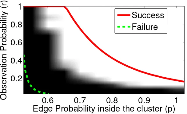
Figure 2.3: Region of success (white region) and failure (black region) of Program 2.1.4 with λ = 1.01D−_min1 . The solid red curve is the threshold for success (λ <

Λsucc) and the dashed green line which is the threshold for failure (λ > Λfail) as

predicted by Theorem1.

p≈ O(polylog_n (n))for success which is order-wise better, and matches closely to the results in McSherry [McS01]. Intuitively, clustering a fully observed graph with pa-rameterspˆ=rp+ 1−randqˆ=rq+ 1−ris much more difficult than one withrp andrq, since the links aremore noisyin the former case. Therefore,while it is bene-ficial to leave the unobserved entries blank in Program2.1.4, for Program2.1.7it is in fact beneficial to set the unobserved entries to0. So, the modified program would have the following sufficient condition for success of Program2.1.7by setting the unobserved entries to0as follows:

min

1≤i≤Krni(pi−q)>2r

√

nprq(1−rq) + 2rmax

1≤i≤K

√

ni p

rpi(1−rpi) +rq(1−rq).

2.3.3 Planted Clique Problem

A fundamental problem related to the hardness of clustering is the planted clique

problem. Consider an Erdös-Réyni random graph1with edge probability 1₂. A sub-set of nodes in this graph is picked and all of them are connected to each other to obtain a clique. Given such a graph (the identity of the nodes that form the clique are unknown), the question of interest is whether we can find the clique efficiently (in polynomial time). The planted clique problem is well-studied in the theoretical computer science community and to the best of our knowledge the tightest result 1_{An Erdös-Rényi random graph on}_n_{nodes with parameter} _p_{is a random graph where each}

(41)

Minimum Cluster Size

Observation Probability (r)

50

100

150

200

0.2

0.4

0.6

0.8

1

Success

Failure

Figure 2.4: Region of success (white region) and failure (black region) of Program 2.1.4 with λ = 1.01D−_min1 . The solid red curve is the threshold for success (λ <

Λsucc) and the dashed green line which is the threshold for failure (λ > Λfail) as

predicted by Theorem1.

(without any unknown constants) is provided in [DM15] where the sufficient con-dition on the size of the clique (number of nodes in the clique) for recovering it successfully is

nmin >

r n

e ≈0.61

√

n,

using asymototic message passing analysis tailored for the planted clique problem. In contrast, the planted clique problem is a special case for the SBM, where the number of clusters K = 1, the edge density inside the clusters is p = 1 and the edge density between he clusters q = 1₂. Thus, by plugging in these parameters in our exact recovery conditions we obtain the following sufficient condtion on the size of the planted clique for its exact recovery,

nmin >2

√

n.

2.4 Experimental Results

We implement Program 2.1.4 and 2.1.7 using the inexact augmented Lagrange method of multipliers [LCM10; LLS11]. Note that this method solves the Pro-gram2.1.4and2.1.7approximately. Further, the numerical imprecisions will pre-vent the entries of the output of the algorithms from being strictly equal to 0 or

(42)

Observation Probability (r)

Edge Probability inside the cluster (p)

0.2

0.4

0.6

0.8

1

0.2

0.4

0.6

0.8

1

Success

Figure 2.5: Region of success (white region) and failure (black region) of Program 2.1.7withλ = 0.49 ˜Λsucc. The solid red curve is the threshold for success (D˜min >

lambda−1_{) as predicted by Theorem}_2.

0.2

0.4

0.6

0.8

1

0

0.5

1

Edge Probability inside the clusters (p)

Probability of Success

Simple

Improved

Figure 2.6: Comparison range of edge probabilitypfor Simple Program2.1.4and Improved Program2.1.7.

each entry. That is, if an entry is less than the threshold, it is rounded to 0and to

1otherwise. We compare the output of the algorithm after rounding to the optimal solution (L0_{), and declare success if the number of wrong entries is less than}₀_._1%_.

Set Up: We consider at an unweighted graph on n = 600 nodes with 3 disjoint

clusters. For simplicity the clusters are of equal sizen1 = n2 = n3, and the edge

probability inside the clusters are samep1 = p2 = p3 = p. The edge probability

(43)

All the results are an average over20experiments.

2.4.1 Simulations for Simple Convex Program

Dependence betweenrandp: In the first set of experiments we keepn1 =n2 =

n3 = 200, and varypfrom0.55to1andrfrom0.05to1in steps of0.05.

Dependence between nmin and r: In the second set of experiments we keep the

edge probability inside the clusters fixed,p = 0.85. The cluster size is varied from

nmin = 20tonmin = 200in steps of 20andr is varied from0.05to1 in steps of

0.05.

In both the experiments, we set the regularization parameter λ = 1.01D−_min1 , en-suring that Dmin > 1/λ, enabling us to focus on observing the transition around

Λsucc and Λfail. The outcome of the experiments are shown in the Figures2.3 and

2.4. The experimental region of success is shown in white and the region of failure

is shown in black. The theoretical region of success is above the solid red curve (λ < Λsucc) and the region of failure is below the dashed green curve (λ > Λfail).

As we can see, the transition indeed occurs between the two thresholdsΛsucc and

Λfail.

2.4.2 Simulations for Improved Convex Program

We keep the cluster size, n1 = n2 = n3 = 200 and varyp from 0.15 to1 and r

from0.05to1in steps of0.05. We set the regularization parameter,λ = 0.49 ˜Λsucc,

ensuring thatλ <Λ˜succ, enabling us to focus on observing the condition of success

around D˜min. The outcome of this experiment is shown in the Figure 2.5. The

experimental region of success is shown in white and the region of failure is shown in black. The theoretical region of success is above solid red curve.

Comparison with the Simple Convex Program: In this experiment, we are

in-terested in observing the range ofpfor which the Programs2.1.4 and2.1.7work. Keeping the cluster size n1 = n2 = n3 = 200 and r = 1, we vary the edge

(44)

Matrix Recovered by Simple Program

100 200 300 400 50

100

150

200

250

300

350

400

450

(a)

Matrix Recovered by Improved Program

100 200 300 400 50

100 150

200

250 300

350

400 450

[image:44.612.119.497.78.268.2]

(b)

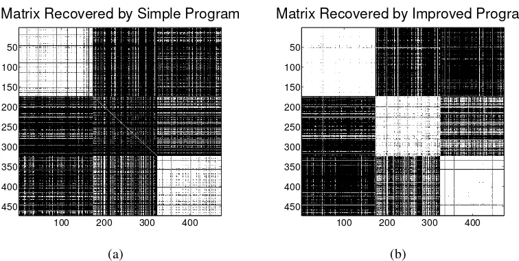
Figure 2.7: Result of using (a) Program2.1.4(Simple) and (b) Program2.1.7 (Im-proved) on the real data set.

Ideal Clusters

50 100 150 200 250 300 350 400 450

0.5 1 1.5

Clusters identifyed by k−means on A

50 100 150 200 250 300 350 400 450

0.5 1 1.5

Clusters Identified from Simple Program

50 100 150 200 250 300 350 400 450

0.5 1 1.5

Clusters Identified from Improved Program

50 100 150 200 250 300 350 400 450

0.5 1 1.5

Figure 2.8: Comparing the clustering output after running Program2.1.4and Pro-gram2.1.7with the output of applying k-means clustering directly onA(with un-known entries set to 0).

2.4.3 Labeling Images: Amazon MTurk Experiment

[image:44.612.147.469.339.508.2]

(45)

A relatively reasonable task is to ask the workers to compare pairs of images, and for each pair, answer whether they think the dogs in the images are of the same breed or not. If we havenimages, then there are n₂distinct pairs of images, and it will pretty quickly become unreasonable to compare all possible pairs. This is an example where we could obtain a subset of the data and try to cluster the images based on the partial observations.

Image Data Set: We used images of3 different breeds of dogs : Norfolk Terrier (172 images), Toy Poodle (151 images), and Bouvier des Flandres (150 images) from the Standford Dogs Dataset [Kho+11]. We uploaded all the 473 images of dogs on an image hosting server (we used imgur.com).

MTurk Task: We used Amazon Mechanical Turk [BKG11] as the platform for

crowdsourcing. For each worker, we showed30pairs of images chosen randomly from the n₂possible pairs. The task assigned to the worker was to compare each pair of images, and answer whether they think the dogs belong to the same breed or not. If the worker’s response is a “yes”, then there we fill the entry of the adjacency matrix corresponding to the pair as1, and0if the answer is a “no”.

Collected Data: We recorded around 608responses. We were able to fill 16,750

out of111,628 entries inA. That is, we observed15% of the total number of en-tries. Compared with true answers (which we know a priori), the answers given by the workers had around23.53%errors (3941out of16750). The empirical parame-ters for the partially observed graph thus obtained are shown Table2.1.

We ran Program2.1.4and Program2.1.7with regularization parameter,λ= 1/√n. Further, for Program 2.1.7, we set the size of the cluster region, Rto 0.125 times

n

2

(46)

val-0 200 400 600 −10

0 10 20 30

A

0 200 400 600

−100 0 100 200 300

Simple

0 200 400 600

−100 0 100 200 300

[image:46.612.222.396.388.450.2]

Improved

Figure 2.9: Plot of sorted eigen values for (1) Adjacency matrix with unknown en-tries filled by0, (2) Recovered adjacency matrix from Program2.1.4, (3) Recovered adjacency matrix from Program2.1.7

Table 2.1: Empirical Parameters from the real data. Params Value Params Value

n 473 r 0.1500

K 3 q 0.1929

n1 172 p1 0.7587

n2 151 p2 0.6444

n3 150 p3 0.7687

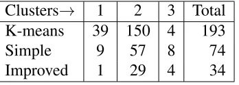
Table 2.2: Number of miss-classified images Clusters→ 1 2 3 Total

K-means 39 150 4 193

Simple 9 57 8 74

Improved 1 29 4 34

ues are very easily distinguished from the rest for the matrix recovered after running Program2.1.7.

A sample of the data is shown in Figure 2.10. We observe that factors such as color, grooming, posture, face visibility, etc. can result in confusion while compar-ing image pairs. Also, note that the ability of the workers to distcompar-inguish the dog breeds is neither guaranteed nor uniform. Thus, the edge probabilities inside and outside clusters are not uniform. Nonetheless, Programs2.1.4and Program 2.1.7, especially Program2.1.7, are quite successful in clustering the data with only15%

observations.

2.5 Outline of the Proofs

(47)

Norfolk Terrier Toy Poodle Bouvier des Flandres

Figure 2.10: Sample images of three breeds of dogs that were used in the MTurk experiment.

2.5.1 Proof Outline for Theorem1

We prove Theorem1by proving the following two lemmas:

Lemma 2.5.1. Ifλ >ΛfailorDmin < _λ