Essays in Behavioral Decision Theory

Thesis by

Matthew L. Kovach

In Partial Fulfillment of the Requirements for the Degree of

Doctor of Philosophy

California Institute of Technology Pasadena, California

2015

Acknowledgements

I am especially grateful for the guidance and encouragement of Federico Echenique and Pietro Ortoleva. I also benefited greatly from discussions with Kota Saito, Jakša Cvitani�, Leeat Yariv, Colin Camerer, John Ledyard, and Marina Agranov.

Abstract

This thesis studies decision making under uncertainty and how economic agents re-spond to information. The classic model of subjective expected utility and Bayesian updating is often at odds with empirical and experimental results; people exhibit systematic biases in information processing and often exhibit aversion to ambigu-ity. The aim of this work is to develop simple models that capture observed biases and study their economic implications.

In the first chapter I present an axiomatic model of cognitive dissonance, in which an agent’s response to information explicitly depends upon past actions. I introduce novel behavioral axioms and derive a representation in which beliefs are

The second chapter characterizes a decision maker withstickybeliefs. That is, a decision maker who does not update enough in response to information, where enough means as a Bayesian decision maker would. This chapter provides ax-iomatic foundations for sticky beliefs by weakening the standard axioms of dynamic consistency and consequentialism. I derive a representation in which updated be-liefs are a convex combination of the prior and the Bayesian posterior. A unique pa-rameter captures the weight on the prior and is interpreted as the agent’s measure of belief stickiness or conservatism bias. This parameter is endogenously identified from preferences and is easily elicited from experimental data.

Contents

Acknowledgements iv

Abstract v

1 Twisting the Truth: A Model of Cognitive Dissonance and

Infor-mation 1

1.1 Introduction . . . 1

1.1.1 The Psychology of Cognitive Dissonance . . . 4

1.1.1.1 Experimental Evidence . . . 5

1.1.1.2 Empirical Evidence . . . 6

1.1.2 Relation to the Literature . . . 6

1.2 Setup and Foundations . . . 10

1.2.1 Formal Setup . . . 10

1.3 Axioms . . . 12

1.3.1 The Standard Axioms . . . 12

1.3.2 Behavioral Axioms. . . 15

1.4 The General Representation . . . 16

1.4.1 Representation and Uniqueness . . . 18

1.5 Proportional Distortions . . . 19

1.5.1 Examples . . . 22

1.6.1 Interpretations . . . 25

1.6.2 Characterization . . . 26

1.7 Connecting the Two Cases. . . 29

1.8 Comparative Dissonance . . . 31

1.9 Applications . . . 32

1.9.1 A Simple Asset Pricing Problem . . . 32

1.9.1.1 Asset Pricing Without Dissonance: Rational Bench-mark . . . 32

1.9.1.2 Prices with Cognitive Dissonance and a Naive Agent 32 1.9.1.3 Prices with Cognitive Dissonance and Sophisticated Agent . . . 33

1.9.2 Response to Information . . . 35

1.9.3 Polarization . . . 36

1.9.4 Purchase of Safety Equipment . . . 38

1.10 Conclusion . . . 40

2 Sticky Beliefs: A Characterization of Conservative Updating 41 2.1 Introduction . . . 41

2.2 Model . . . 45

2.2.1 Setup . . . 45

2.2.2 Axioms . . . 46

2.2.3 Novel Axioms . . . 48

2.3 Main Results . . . 49

2.4 Conclusion . . . 51

3 Partial Bayesian Updating Under Ambiguity 52 3.1 Introduction . . . 52

3.2 Related Literature . . . 56

3.3 Preliminaries and Notation . . . 58

3.3.1 TheUnambiguously PreferredRelation . . . 58

3.4 Model . . . 59

3.4.1 Objective Randomizations . . . 62

3.4.2 Example 2 . . . 64

3.5 Additional Properties ofα-BU . . . 66

3.5.1 Informational Path Independence . . . 66

3.5.2 Comparative Inference and Completeness . . . 66

3.6 Conclusion . . . 68

A Appendix to Chapter 1 69 A.1 Best-Case Binary Distortion: δ(A, f)Comparative Statics . . . 69

A.2 Preliminary Results . . . 72

A.3 Proofs . . . 75

A.3.1 Proof of Theorem 1.1. . . 75

A.3.2 Proof of Theorem 1.2 . . . 78

A.3.3 Proof of Theorem 1.3 . . . 79

A.3.4 Proof of Theorem 1.4 . . . 82

A.3.5 Proof of Theorem 1.5 . . . 82

A.3.6 Proof of Theorem 1.7 . . . 89

A.3.7 Proof of Theorem 1.9 . . . 90

B Appendix to Chapter 2 91 B.1 Proof of Theorem 2.1. . . 92

B.2 Proof of Theorem 2.2 . . . 97

C Appendix to Chapter 3 99 C.1 Proof of Theorem 3.1. . . 99 C.2 Proof of Theorem 3.3 . . . 102

List of Figures

1.1 States and Information . . . 14

1.2 Scenarios(A, f)and(B,g). . . 20

1.3 Indifference curves for≿_A,f. . . 27

1.4 Predicted price paths for f = (1, 3, 4, 6) and (i) the agent is ratio-nal (blue dashes),(ii)a naive agent experiences cognitive dissonance, δ = 1₂ (red), and(iii)a sophisticated agent experiences cognitive dis-sonanceδ = 1₂(purple) . . . 34

1.5 Indifference curves for≿1_A,f and≿2_A,g.. . . 38

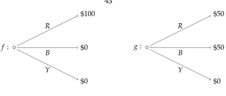
2.1 Two acts,f andg. . . 43

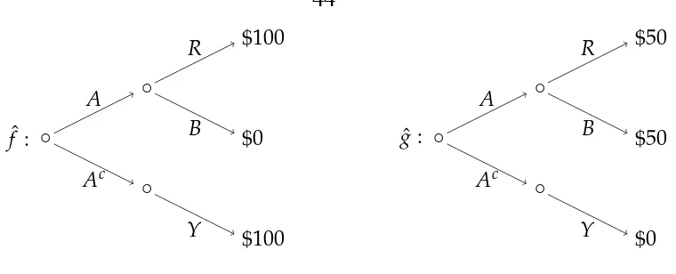
2.2 Two acts,fˆandgˆ, incorporating information. . . 44

2.3 Dynamic extension of f andg . . . 47

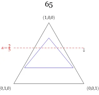
3.1 Sets of beliefs in the simplex. . . 61

3.2 The set of posterior beliefs,C_Cα, asαvaries. . . 65

Chapter 1

Twisting the Truth: A Model of Cognitive

Dissonance and Information

1.1

Introduction

This paper provides a theory of how an agent sensitive to cognitive dissonance in-corporates new information into his beliefs. Cognitive dissonance refers to the psy-chological discomfort that arises when twocognitionsare in conflict. In this paper, cognitive dissonance arises when information and a previous action are in conflict. That is, if the agent updated his beliefs according to Bayes’ rule, his beliefs and past actions would create dissonance. The agent assuages this cognitive dissonance by incorporating information in a non-Bayesian manner and distorting his beliefs to support his previous actions.

an inherent desire to justify past actions. This paper investigates how the agent resolves the tension between Bayesian learning and the desire to view past actions as optimal.

As a simple example, consider an investor deciding which company’s stock to purchase. After the investor makes his initial purchase, he receives some infor-mation that is relevant to the company’s valuation. The investor now must take the new information into account and decide again which stocks to purchase (or sell). However, our investor is sensitive to cognitive dissonance and thus experi-ences psychic distress if the new information, combined with his original beliefs, suggests that he originally made a poor investment decision. Hence the investor’s original decision and new information jointly determine his updated beliefs, and consequently his new decision.

While the concept of cognitive dissonance is well known, the psychology liter-ature has not provided a precise notion of how it affects an agent’s future deci-sion making, which is necessary to apply the model to economic problems. The main contribution of this paper is to answer these questions in a way suitable for an economist. I utilize a standard economic setup to study the effect of informa-tion on preferences. Within this framework I introduce behavioral condiinforma-tions, in the form of axioms on preferences, that capture cognitive dissonance and then de-rive a utility representation. Thus this paper answers the question of how cognitive dissonance affects an agent’s response to information.

this axiom, consider an investor that invests in companyXat time 1. In particular, suppose companyXmay either yield a high return or a low return. SayHandLare the events in which X provides a high or low return, respectively. Then after any observation, at time 2 the agent prefers investments that also have high payoffs in H. The resulting utility representation is one in which the agent’s time 2 beliefs

shift probability from states in which the time 1 action, denoted by f, is relatively poor to states in which it is relatively good.

In addition to the general model I characterize two special cases, each of which is derived by imposing one additional axiom. The first case I characterize is the pro-portionaldistortion. Under this representation the agent distorts the relative likeli-hood between states by the payoff of f in those states. Thus it is as if the agent views his original action f as being informative about the relative likelihood of states of the world. The proportional distortion is characterized by the addition of ascenario independenceproperty, which states that whenever two scenarios share a common event in which each action provides the same state-wise payoff on the common event, then the agent’s ranking of acts that vary only on the common event are the same in each scenario. That is, the relative distortion between any two states is independent of the payoffs in any other states.

weight that each self receives in the representation is endogenously captured by a unique parameter,δ, which I interpret as the agent’s sensitivity to cognitive disso-nance. An agent that is very sensitive to dissonance, or has a largeδ, puts greater weight on the justifying states.

The model produces some interesting, testable implications. First, risk free actions induce no belief distortion and thus the agent appears Bayesian in some situations. This is intuitive since there is no payoff variation in a risk free action and hence there is no possible revision of beliefs that could make the action ap-pear better. Second, the agent will exhibit an asymmetric reaction to good and bad news, which is consistent with empirical evidence on financial analysts’ forecasts (see Easterwood and Nutt, 1999). That is, if we consider an agent’s monetary valu-ation of some action, the agent always overvalues the time 1 action compared to a Bayesian agent. Thus the agentover-reactsto the good news andunder-reactsto the bad news. Neither of these implications can result from models of non-Bayesian updating that do not also condition on an agent’s past action.

1.1.1

The Psychology of Cognitive Dissonance

The theory of cognitive dissonance, developed by Leon Festinger [22], states that people tend to adjust beliefs to enhance the attractiveness of their past actions. In particular, Festinger proposed that conflict or tension between beliefs and actions creates psychological discomfort. He termed this resulting discomfortdissonance

and states that the only way to eliminate this discomfort is to eliminate the conflict and achieve consonance. Thus after taking some action people are motivated to change their beliefs about the desirability of that action.

following conflicting thoughts, I bought X expecting high returnsand this infor-mation suggestsXwas a bad investment, and hence suffers the discomfort caused by cognitive dissonance. In order to achieve consonance the agent incorporates the new information into his original beliefs in a biased manner. This bias causes the agent to increase the conditional likelihood of high returns and hence to view investment inXmore favorably than an outside Bayesian would.

1.1.1.1 Experimental Evidence

In an early and influential laboratory experiment, Festinger and Carlsmith [23] asked students to perform a long and boring task and then to recruit more par-ticipants. Some students were paid a substantial amount while others were paid very little. Those who were paid very little reported the task as more interesting than students who were paid a more substantial amount. This suggests that those who were paid little manipulate their beliefs in order to justify performing the task for very little pay. Similarly, students who gave speeches advocating an ideological position were more likely to align their beliefs with their speech the lower their pay (see Aronson [5] for an overview of this and other experiments).

proba-bility and for the Bayesian posterior of the subject’s reported beliefs from previous periods. This suggests that subjects update their beliefs in a non-Bayesian manner dependent on their actions.

1.1.1.2 Empirical Evidence

The specific role of cognitive dissonance in voter preferences was studied by Mul-lainathan and Washington [49]. They measured the effect of voting for a candidate on a voter’s future opinion of that candidate. To control for the selection problem, the authors compared the opinion ratings of voting age eligible and ineligible vot-ers two years after the 1996 presidential election. They found that eligible votvot-ers showed 2-3 times greater polarization than ineligible voters, supporting the rele-vance of cognitive dissonance in shaping political attitudes.

A more recent paper by Kaplan and Mukand [37] shows that political party reg-istration seems to be excessively persistent. They also utilize a discontinuity design based on voting age while also utilizing the 9/11/01 terrorist attacks as an exogenous shock to party registration. Party registration is persistent even for those registered near universities, suggesting that this persistence is not easily explained by lack of access to information.

1.1.2

Relation to the Literature

Akerlof and Dickens [2] developed perhaps the earliest model of cognitive disso-nance in economics. They allow for the agent to choose his beliefs while consider-ing both the cost of makconsider-ing the wrong decision and a psychological cost of believ-ing that his past choice was suboptimal.1 Their main result shows that cognitive

dissonance may cause workers to forgo efficient safety equipment. An application demonstrating that this result generally holds is developed later in the paper.

Perhaps the most closely related papers are Yariv [63] and Epstein and Kopylov

[18]. Yarivconsiders as a primitive preferences over pairs of actions and beliefs.

She then provides axiomatic foundations for a linear representation over infinite streams of action and beliefs pairs. However, her setup and axioms do not deliver any specific way in which actions and beliefs interact. Additionally, it may be that the action has no impact on the next periods belief. Epstein and Kopylovconsider a model with preferences over menus of acts and impose modifications of the Gul and Pesendorfer [32] axioms. They derive a representation where the agent chooses a menuex-anteto balance his preferences under commitment—expected utility with respect to true beliefs—with a temptation utility—where the agent minimizes (or maximizes) the value of an action over a set of priors. While conceptually similar, [18] is distinct in two important ways. First, the representation suggests ex-post

choice from the menu is of a max-min form while this paper imposes expected util-ity. Second, the set of priorsQis independent of any choices the agent makes and hence ex-post beliefs are independent of the agent’s actions, while in this paper posterior beliefs explicitly depended upon the agent’s action.

Mayraz [46] studies a model of payoff-dependent beliefs. His paper assumes preferences conditional on some real-valued payoff function, but does not have a notion of ex-ante vs ex-post preferences or information and thus does make the connection to non-Bayesian updating or weakening dynamic consistency. Addi-tionally, he requires distortions to take a specific functional form, whereas this pa-per studies a general model that allows for a variety of distortions.

non-Bayesian behavior (consequences of which are explored in [21]) but does not allow for updating to depend on anything other than the information received. In contrast I propose a single behavioral axiom, along with some regularity conditions, and generate a representation such that updated beliefs depend explicitly upon past choice.

Ortoleva [52] develops an axiomatic model of updating that is at the intersection of Bayesian and non-Bayesian models. That is, he introduces thehypothesis testing representationwhich holds whether or not the agent utilizes Bayes’ rule to update beliefs. However, the Bayesian model is embedded as a special case. An agent in his model chooses a new prior only in the case of an unexpected (low probability) event, and may or may not use Bayes’ rule otherwise. The model presented in this paper is distinct since the deviation from Bayes’ rule depends on the interaction of a past choice and information, not purely on information. Thus an agent in this model can behave as a Bayesian when responding to an unexpected event and violate Bayes’ rule for an expected event.

A closely related, non-axiomatic paper is Yariv [64]. She considers an agent represented by an instrumental utility (a classical utility over consequences) and a belief utility, where the belief utility captures the agent’s innate preference for be-lief consistency. Her agent is forward looking, though the agent may incorrectly forecast the weight placed on the belief utility. However, in each period the agent’s choice is over beliefs, subject to the constraint that the agent will take an action con-sistent with his beliefs and suffers a cost of changing his beliefs. This is contrasted with my model in which the belief change is not necessarily a conscious procedure and manipulations force beliefs to bemoreconsistent with past actions, rather than past beliefs. (see also Bénabou and Tirole [9], Bénabou [8]).

utility is defined over both prizes and psychological states. However, the model designed to study the role ofanticipatoryfeelings. Such an agent chooses his be-liefsex-anteto balance hisinstrumental(prize) utility and his utility from antici-pation (anxiety). Thus their model is not well suited to study cognitive dissonance, since cognitive dissonance is not a forward looking emotion but a retrospective one.

Brunnermeier and Parkerconsider a dynamic model in which the agent balances

how much he distorts his beliefs from the truth with his taste for optimistic expec-tations about future utility. Once the initial belief is chosen however, the agent acts as a Bayesian in all future periods. [31, see also]

A psychological concept closely related to cognitive dissonance is motivated reasoning. An agent engaging in this behavior reasons so that he may support his favored ideas or actions, perhaps by only acknowledging some information (see Kruglanski [42] Kunda [44]). In a sense, motivated reasoning can be seen as a mechanism by which cognitive dissonance is reduced. With this view, the model of cognitive dissonance in this paper is also a model of motivated reasoning. Moti-vated reasoning in political science has been studied by Redlawsk [57] and by Taber and Lodge [62].

within an event. The literature on alternatives to the Bayesian model is perhaps larger; for a sample, see Camerer [11], Kahneman and Tversky [36], Mullainathan et al. [50], Rabin and Schrag [55], Rabin and Vayanos [56].

1.2

Setup and Foundations

1.2.1

Formal Setup

I adopt a standard setup for studying the effect of information on preferences. There is a finite setSof states of the world, with |S| ≥ 3.2 Events are denoted A,B,C ∈

Σ = 2S\{S,∅}3 and X denotes the set of consequences, assumed to be a convex subset of a vector space. For example, Xcould be the set of monetary prizes (e.g. X = R+) or X could be the set of lotteries over some setY (which corresponds to

the classic Anscombe–Aumann setup [4]). LetF denote the set of all acts, which are functions f : S → X. Following a standard abuse of notation, let x ∈ F de-note the constant act that returnsx ∈ Xin every state. For any event Aand acts f,g ∈ F, let f Agdenote the acthsuch thath(s) = f(s)fors ∈ Aandh(s) = g(s) fors ∈ Ac.

Let ∆(S) denote the set of probability distributions over S, which is identified with the|S| −1dimensional simplex inR|S|. For anyµ ∈ ∆(S)and anyA ∈ Σ, let

µ_|A(or sometimesµ(·|A)) denote the Bayesian update ofµgivenA4.

Definition 1.1 (Scenario). I will refer to an information-choice pair, (A, f), as a

scenario.

I take as a primitive a class of preference relations{≿,≿A_,f}(A,f)∈Σ×F overF.

2_{The assumption of finiteSis merely for convenience. All results are unchanged if I assume an} infinite state space and restrict attention to non-null events. What is crucial is the existence of at least three non-null events.

3_{I assume that the agent’s information is in fact informative.} 4_{That is, for allB∈Σ,µ(B|A) =} µ(B∩A)

Here≿represents the agent’sex-antepreferences, while≿A_,f is interpreted as his preference after making choice f and receiving information A; his preferences in scenario(A, f).5

The literature offers two interpretations for conditional preferences: 1) ≿_A,f represents what the agent thinks his preferences would be if he later faced scenario (A, f); and2)≿_A,f are his actual preferences when facing scenario(A, f). For this paper I adopt the second interpretation and assume that≿_A,f is a representation of how the agent actually respondsex-postin scenario(A, f).

The statement h ≿A_,f gmay be interpreted as follows: after having chosen f and learning A, the agent prefers h to g. In this way preference statements may be connected to choice data by observing choices from binary menus.6 Thus the primitives may be interpreted as follows (i) at time 1 the experimenter elicits the agent’s preferences, then (ii) during an interim period the agent chooses an alter-native and then receives information, and finally (iii) at time 2 the experimenter elicits the agent’s preferences again. The interim choice is not modeled and could be made from some subset of acts (a menu) or possibly utilize some form of ran-domization.7

5_{Alternatively, I could simplify notation by writing the above conditions only in terms of≿}

A,f, for A∈Σ∗ =Σ∪S, and imposing the condition that≿_S,f=≿_{S, ˆf}, for allf, ˆf, in which case we identify≿ with≿_S,f. This changes the interpretation of the model, in that I interpret≿as preferences before both information and choice, whereas in the new formulation all preferences are conditional on some action. However, it is reasonable to argue that even in the presence of cognitive dissonance, if no new information is received, (i.e., the agent observesS) then the fact that a choice was made does not immediately impact preferences. That is, I argue that dissonance requires information. Additionally, the fact that the model implicitly assumes≿_S,f=≿_{S, ˆf} makes for a clear distinction between the model here and models of status-quo bias.

6_{It is simple to translate the framework and axioms into an inter-temporal choice setting. I utilize} preferences as a primitive for axiomatic transparency.

1.3

Axioms

1.3.1

The Standard Axioms

The first axiom,Consistent Expected Utility, is a collection of classic axioms which are known to be equivalent to subjective expected utility maximization, plus ordinal preference consistency, which is a regularity condition between theex-anteand ex-post preferences. Ordinal preference consistency is sensible in this environment, even in the presence of cognitive dissonance. In particular, suppose X is a set of monetary prizes, say[0, 10]. Then the condition merely imposes that if$10is pre-ferred to$1before information, it is also preferred after information, regardless of what the agent has done in the past.

Axiom 1.1(Consistent Expected Utility). For all A∈ Σandg,h, f, ˆf ∈F.

Weak Order: ≿and≿A_,f are complete and transitive binary relations on

F.

Independence:For allα ∈ (0, 1).

(i) f ≿gif and only ifαf + (1−α)h≿αg+ (1−α)h. (ii) f ≿_{A, ˆf} gif and only ifαf + (1−α)h≿_{A, ˆf} αg+ (1−α)h.

Strict Monotonicity: Ifh(s) ≿ g(s)for alls, thenh ≿g. In addition, if for somes, h(s) ≻ g(s), then h ≻ g. Similarly, if h(s) ≿_A,f g(s) for alls, then h≿_A,f g, and if in additionh(s) ≻_A,f g(s)for somes, thenh ≻_A,f g.

Continuity: The sets {α ∈ [0, 1] : αf + (1−α)g ≿ h},{α ∈ [0, 1] : h ≿

αf + (1−α)g},{α ∈ [0, 1] : αf + (1−α)g ≿_{A, ˆf} h} and{α ∈ [0, 1] : h ≿_{A, ˆf}

αf + (1−α)g}are closed.

Non-triviality: There arex,y∈ Xsuch thatx ≻y.

Consequentialism is also a standard axiom, which ensures that the agent be-lievesthe information. That is, once the agent learns states outside ofAare impos-sible, he is only concerned with how actions perform within A. That is, the agent’s posterior beliefs put probability 1 onA.

Axiom 1.2(Consequentialism). For all A∈ Σand f ∈ F,

h(s) = g(s)for alls∈ A =⇒ h∼_A,f g.

The novel axioms will be concerned withhowthe agent changes his preferences after receiving information. Before introducing them I first introduce another clas-sic axiom.

Axiom 1.3(Dynamic Consistency). For allh,g∈ F and A∈ Σ,

hAg≿g⇐⇒ h≿_A,f g.

This axiom requires that the ranking of two acts, after the arrival of information A, only depends on their variation in Aand is consistent with the agent’sex-ante

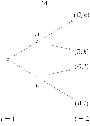
ranking between acts that only vary within A. In other words, the agent does not adjust the relative probabilities of states in A. While the axiom has normative ap-peal, it is too restrictive and rules out any sensitivity to cognitive dissonance. In particular, an agent sensitive to cognitive dissonance allows yesterday’s action to influence today’s preferences. However, dynamic consistency requires preferences to be independent of yesterday’s action. The following example illustrates this. Example 1.1(Investing). Consider an example similar to the experimental setup in [43]. An investor is deciding between a stock,s, and a bond,b. The stock can be

.. ◦.

◦ .

L .

◦

.

H

.

(B,l) .

(G,l) .

(G,h)

. (B,h)

.

t = 1

.

t =2

Figure 1.1: States and Information

stock can pay either a high or low dividend. Good stocks are more likely to pay high dividends.

Formally, the state space isS={(G,h),(G,l),(B,h),(B,l)}andµis the agent’s prior. Suppose that good and bad are equally likely but a high dividend correlates with a good stock—µ(G,h) =µ(B,l) = 3₈ andµ(B,h) =µ(G,l) = 1₈.8 LetH(L)be the event that a high (low) dividend is observed.

If agents satisfy dynamic consistency, then µ_H,s(G) = µ_H,b(G). However, the experimental evidence finds that subjects report µ_H,s(G) > µ_H,b(G). Formulated in terms of observables, we can consider preferences between two the following two bets:

(G,h) (B,h) (G,l) (B,l)

f $3 $0 $0 $0

g $0 $9 $0 $0

Before the dividend is observed the agent is indifferent between the two bets, f ∼ g. Dynamic consistency requires the agent to also be indifferent after the

idend observation—f ∼H,s g and f ∼H,b g—regardless of which asset the agent

originally choose. However after observing the dividend, the stock holder is more optimistic than the bond holder and thus we expect f ≻_H,s g, a violation of dynamic consistency

1.3.2

Behavioral Axioms

As seen inExample 1.1,Dynamic Consistencyis too strong and rules out cognitive dissonance. This is because it requires that both those that voted for the hawk and those that voted for the dove have the same posterior after observingA. It requires that relative likelihoods between states are constantand independent of prior ac-tions, whereas cognitive dissonance implies that relative likelihoods change in favor ofstates that favor prior actions. The following behavioral axiom,Dynamic Cog-nitive Dissonance, is the precise weakening ofAxiom 2.2needed for the behavior seen inExample 1.1.

Axiom 1.4 (Dynamic Cognitive Dissonance). For all (A, f) and B,C ⊂ A, such that for everys ∈ Bands˜∈ C, f(s)≿ f(s), then for any˜ x,y,z∈ X, wherex,y≿z,

xBz≿yCz =⇒ xBz ≿_A,f yCz.

Axiom 1.4states that for any pair of events, where one event is always better ac-cording to the previous action, the agent weakly prefers to bet on the better event. That is, think about an agent committed to action f. This induces a preference over what events might occur, where the agent preferss tos˜if f(s) ≻ f(s). Since cog-˜

nitive dissonance causes the agent to align his conditional beliefs with f, if he were to learn that{s, ˜s}has occurred he ought to prefer betting onstos. In the context˜

peace if he voted for the dove. Since agents are expected utility maximizers, such a belief distortion will cause the agent to support more extreme policy positions in future elections.

1.4

The General Representation

This section introduces the main model for cognitive dissonance. I discuss sev-eral properties of the gensev-eral model and then present a representation theorem, showing that the model is equivalent to some standard postulates and the behav-ioral weakening ofDynamic Consistency—Dynamic Cognitive Dissonance. I then discuss the model’s uniqueness properties.

Definition 1.2(Cognitive Dissonance Representation). There exists utility func-tionu: X→R, a prior beliefµ ∈ ∆(S), and for each(A, f), an increasing distortion functionδ_A,f : u(X)→R+such that

≿is represented by:

V(g) =

∑

s∈S

u(g(s))µ(s),

≿A,f is represented by:

V_A,f(g) =

∑

s∈A

u(g(s))µ_A,f(s),

where

µA,f(s) =δA,f(u(f(s)))µ(s|A).

magni-tudes may vary considerably between scenarios, even if state-wise payoffs are iden-tical. This scenario sensitivity may or may not be sensible in certain contexts, both of which will be explored later. This model embeds the standard Bayesian model as a special case, whereδ_A,f(a) =1for all a∈ u(X).

To clarify, the agent does not privilege the past choice, f, per se. Rather, he privileges those states of the world in which, given the partition he finds himself in, his past choice would do best. Thus the agent may in fact move away from f after information. That is, he views f as a commitment to certain states of the world and hence his beliefs become biased in favor of those states. Alternatively, one may interpret this as if the agent views his action f as an additional piece of informa-tion and uses this informainforma-tion to adjust the relative probabilities of statess ∈ A. This last interpretation is reminiscent of Bénabou and Tirole [9], which considers a model of an agent who infers their beliefs from their past actions.

Consider some scenario(A, f)and suppose f(s) ≿ f(s)˜ for somes, ˜s ∈ A. Then the agent’sex-postsubjective relative likelihood of statesto states˜is given by

µA,f(s)

µA,f(s)

= δA,f(u(f(s)))

δA,f(u(f(s)))˜ ×

µ(s)

µ(s).

Sinceδ_A,f is increasing, and f(s) ≿ f(s), it follows that˜ δ_δA,f(u(f(s)))

A,f(u(f(s˜))) ≥ 1, hence the

agent believes s to berelativelymore likely than s˜when compared to a Bayesian agent.

Notice that if f(s) ∼ f(s), then˜ δ_A,f(u(f(s))) =δ_A,f(u(f(s)))˜ and henceµA,f(s) µA,f(s) = µ(s)

µ(s).Thus the relative likelihood between states that provide identical payoffs under

f is undistorted. This is actually quite intuitive, since whatever feelings the agent has towards, since both statessands˜are equally good according to his action, he should have precisely the same feelings towards.˜

Then regardless of the information he learns, there is no possible distortion of this information that could increase the agent’s valuation ofx, hence there is no distor-tion of beliefs at all. This reasoning extends to all scenarios that are equivalent to having taken a constant action. The following definition precisely identifies which scenarios are equivalent to a constant action.

Definition 1.3. A scenario(A, f)is constant if for alls, ˜s ∈ A, f(s)∼ f(s).˜

A constant scenario is one in which the agent’s initial action does not vary, con-ditional on eventA. Thus conditional onA, there is no distortion of beliefs that can improve the valuation of f. LetC denote the set of constant scenarios.

Observation 1.1. For all(A, f) ∈ C, the agent’s posterior beliefs are derived via

Bayes rule,µ_A,f =µ_|A.

1.4.1

Representation and Uniqueness

This section presents the representation theorem and the uniqueness properties of the representation. The following theorem connects the representation to the axioms.

Theorem 1.1(Representation). The following are equivalent:

(i) {≿,≿_A,f} satisfy Consistent Expected Utility, Consequentialism, Dynamic

Cognitive Dissonance,

(ii) The agent admits aCognitive Dissonance Representation.

we have a unique µ_A,f for every scenario, while uniqueness of δ follows from the decomposition into the productδ_A,f(f(s))µ(s|A).

Theorem 1.2(Uniqueness).If(u,µ,δ_A.f)and(u′,µ′,δ′_A.f)both represent{≿,{≿A_,f

}}then

(i) u′ =αu+βforα >0,β∈R

(ii) µ′ =µ

(iii) δ′_A,f(u′(x)) = δ_A,f(u(x))for allx∈ f(A).

1.5

Proportional Distortions

This section introduces and characterizes the first special case by introducing a sce-nario independence property. While the general representation allows for some arbitrariness between scenarios, it is natural to think that the distortions between any two states should only depend on the relative payoffs between those states. To this end I define the proportional distortion.

Definition 1.4(Proportional distortion). The belief distortion function is a pro-portional distortion if there exists an increasing function v : u(X) → R+ such

that

δA,f(a) :=

v(a)

∑s∈Av(u(f(s)))µ(s|A)

. (1.1)

In the case of a proportional distortion, the belief distortion only depends on the scenario up to a normalizing constant. This becomes clear when looking at the probability ratio of any two states. Suppose f(s) ≻ f(s), then after learning some˜

.. _{f :} . _◦ . ◦ . Ac . ◦ . A . $y . $0 . $x . $50 . s₁ . s2 . s₃ . s4

.. _{g :}

. _◦ . ◦ . B . ◦ . Bc . $z . $0 . $w . $50 . s₁

. s2

.

s₃ .

s4

Figure 1.2: Scenarios(A, f)and(B,g).

Example 1.2. More precisely, supposeS = {s₁,s2,s3,s4}, and consider the

fol-lowing two events A={s₁,s₂,s₃}andB ={s₂,s₃,s₄}and the following two acts: s1 s2 s3 s4

f $x $50 $0 $y

g $w $50 $0 $z

Figure 1.2illustrates scenarios(A, f)and(B,g). SupposeC ={s₂,s3}= A∩B

(shown in blue) and consider the agent’s preferences over acts that vary only within C. More specifically, consider an agent placing bets on a given state, say bets of

the form ($a,s₂)and ($b,s₃). If an agent is in scenario(A, f), then since50 > 0, an agent sensitive to cognitive dissonance may distort the relative probabilities of statess2ands3. It is natural to think that when determining preferences over the

binary bets, theonlyrelevance of f is through how it performs in states s2and s3.

That is, the specific value ofy is irrelevant. If this is the case, then sinceg(s2) =

f(s2)andg(s3) = f(s3), the agent should report the same preferences over binary

bets of the form($a,s₂)and($b,s₃)when in scenario(B,g).

the previous example.

Axiom 1.5(Scenario Independence). For all(A, f),(B,g)andC ⊂A∩B, if f(s)∼ g(s)for alls∈ C, then for allh,j∈ F and anyz∈ X,

hCz≿_A,f jCz ⇐⇒ hCz≿B,g jCz.

For any two scenarios, if there is some event in which both action f and action g are payoff equivalent, then the preference ordering between any two acts that vary only on that event is the same in either scenario. The next theorem shows that the addition ofScenario Independencecompletely characterizes proportional distortions.

Theorem 1.3(Representation). Suppose {≿,≿A_,f} satisfy Consistent Expected Utility,Consequentialism,Dynamic Cognitive Dissonance, then the following are

equivalent,

(i) {≿,≿_A,f}satisfyScenario Independence

(ii) δ_A,f is a proportional distortion

While Theorem 2 shows the uniqueness of δ_A,f, the same uniqueness does not extend to the value function determining a proportional distortion. That is,vis only identified up to the ratio ofδ_A,f(a)andδ_A,f(b), as shown in the following theorem.

Theorem 1.4(Uniqueness). Suppose{≿,≿A_,f}has a cognitive dissonance rep-resentation with a proportional distortion. Then the value functionvis unique up

to a positive scalar.

Axiom 1.6(Commitment Continuity). For allAand allf,g,hFand any(fn),(gn),(hn) ∈ F∞_{such that f}

n → f,gn → g,hn →h:

ifgn ≿A,fn hnfor alln, theng≿A,f h.

As will be shown later however, there is an interesting class of distortions that are not continuous in the sense ofAxiom 1.6.

Corollary 1.1. Suppose{≿,≿A_,f}satisfyConsistent Expected Utility,

Consequen-tialism,Dynamic Cognitive Dissonance,Scenario Independence, then the

follow-ing are equivalent:

(i) The value functionvis continuous

(ii) {≿,≿A,f}satisfyCommitment Continuity

1.5.1

Examples

The following examples may help illustrate the distinction between continuous and discontinuous proportional distortions.

Example 1.3(Step Distortion). Fix a parameter θ ∈ (0, 1)and some a∗ ∈ u(X). Then

v(a) =       

1+θ ifa≥a∗

1−θ ifa<a∗

of gains relative to losses. In this case, any scenario(A, f)that yields only gains or only losses will result in posterior beliefs that coincide with using Bayes’ rule. Non-Bayesian behavior in this example would only be observed when observingmixed

scenarios - those in which(A, f)allows for both gains and losses.

Example 1.4(Logistic Distortion). Fix a parameterλ ∈ [0,∞). Thenv(a) = eλa is a logistic distortion, where

δA,f(u(x)) =

eλu(x)

∑s˜∈Aeλu(f(s˜))µ(s|A)

and the likelihood ratios are given by

µA,f(s)

µA,f(s)˜

= µ(s)

µ(s)˜ e

λ[u(f(s))−u(f(s˜))]

A version of the logistic distortion was studied by Mayraz [46]. The logistic dis-tortion includes the Bayesian model as the special caseλ=0.

Example 1.5 (Distortion with Decreasing Sensitivity). Suppose u(X) = [0,∞). Then definev: u(X) →Rby

v(a) = ln(1+a)

.

1.6

Binary Distortions

While continuity is often considered an attractive property, there are interesting cases in which the distortion is not continuous. For example, the distortion may take the form of a step function. This may be interpreted as an agent separating the event Aintogoodandbad states, and only overweighting the probability of good states relative to bad states. In contrast to the proportional distortion, in which the scenario only matters for a normalization, the class of binary distortions are often most sensible when there is scenario dependence.

That is, the agent determines some threshold depending on (A, f), and states which are better than the threshold are classified asgood. The following definition introduces a special case of the binary distortion.

Definition 1.5(Best-case Binary Distortion). The belief distortion is aBest-case Binary Distortion9if there exists a non-constant, affine utility functionu : X →R, a probability distributionµ ∈ ∆(S), and a functionδ : Σ×F →[0, 1]such that:

≿is represented by:

V(g) =

∑

s∈S

u(g(s))µ(s),

≿A,f is represented by:

V_A,f(g) =

∑

s∈A

u(g(s))µ_A,f(s)

where

µA,f(s) = (1−δ(A, f))µ(s|A) +δ(A, f)µ(s|D(A, f))

9_{This representation fits into the general model as a binary distortion given by the pair(θ,t),} whereθ:Σ×F →[0, 1]andt:Σ×F →Xsuch that

δA,f(x):= {

1−θ(A,f) ifx≺t(A,f)

and

D(A, f) = {s∈ A|f(s) ≿ f(s′)for alls′ ∈ A}.

1.6.1

Interpretations

Here V represents the ex-antepreference and V_A,f represents the agent’s prefer-ences after informationAand the choice off. Behaviorally,δrepresents the agent’s

sensitivity to dissonance. Presented in this form, it looks similar to the “α-maxmin expected utility” model of Arrow and Hurwicz [6]. In a way they are similar, as they both allow the agent to “average” the utility of an act according to a “pessimistic (ra-tional)” belief and an “optimistic” belief. The similarity is only superficial, however, since in this model the agent’s preferences satisfy the subjective expected utility ax-ioms. Hence the agent being studied has beliefs represented by a unique probability distribution over the states, whereµ_A,f(s) = (1−δ)µ_|A(s) +δµ_D(A,f)(s).

guns” by repeating the previous choice.

This representation suggests a specific “cognitive mechanism” that underlies multi-period choice and updating. The agent considers a scenario, an information-choice pair, and partitions the event into good and bad states. As mentioned ear-lier, good states are states in which f performs best given the known information. This is a rather blunt cognitive rule, since even if two states are very close in utility space, they may be classified as “distinct states.” Hence preferences are generally discontinuous between scenarios.

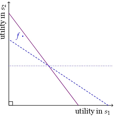
Example 1.6. In order to get a better understanding of how this bias affects pref-erences, consider the following simple example. SayX = [w,b] ⊂Randu(x) = x. SupposeS= {s₁,s2,s3}with priorµ = (1/3, 1/4, 5/12), and suppose A ={s1,s2}

. Consider an act f = (y,x,z), where x ≻ y ≻ z. Then the Bayesian posterior is given by µ_|A = (4/7, 3/7) and the corresponding indifference curve in utility space, illustrated inFigure 1.3, corresponds to the solid line (δ = 0). Sincex ≻ y, thenD(A, f) = {s₂} andµ_|D(A,f) = (0, 1). The horizontal dotted line denotes the indifference curve of an agent that has taken action f with δ = 1, whereas the in-termediate dashed line represents the corresponding indifference curve forδ = 1₂. For clarity, the curves all intersect at the constant utility liney =x.

1.6.2

Characterization

Before introducing the next axiom I first introduce a few definitions. The first is comonotonicity, which is standard in the literature.

..

u

ti

li

ty

i

n

s2

.

utility ins₁ .

f

..

δ =0

.

δ =1/2

.

δ =1

Figure 1.3: Indifference curves for≿A_,f.

Consider an agent that has taken action f and is sensitive to cognitive disso-nance. Then one would expect the agent to express an inflated view about the value of f. However, dissonance theory suggests more than this. That is, the agent will seek out aconsistentview of the world, and hence will similarly express an inflated view about the value of actions that are similar to f. Thus we seek to impose a weak-ening of dynamic consistency that takes into consideration the impact of the action

f on all similar acts. This leads to the following axiom.

Axiom 1.7(Best-Case Dominance). For all A, and allh,g≍A f:

hAg≿g

h(s) ≿g(s′), for somes ∈ Aand alls′ ∈ A    

 =⇒ h ≿A,f g

he would say he was indifferent between taking either action. However, after taking an action and having observed A, the agent feels the need to justify having taken f as opposed to g. Thus we come to the second condition — if the best possible payoff of action f is better than the best possible payoff of action g, then the agent can use that as a justification to declare a preference for f overg. Third, I extend this logic to all actions that are strongly A-comonotonic with f. That is, imagine an agent who is contractually obligated to some action f. Then this commitment to f induces a preference over states of the world. However, an action h that is stronglyA-comonotonic with f induces the same preference over states, and hence in a sense they are equivalent. That is, they induce the same desires abouthow the world turns outand thus if commitment to f induces a dynamic inconsistency, any arguments or justifications used for f also apply to h.

Theorem 1.5(Representation). The following are equivalent:

(i) {≿,≿_A,f} satisfy Consistent Expected Utility, Consequentialism, Dynamic

Cognitive Dissonance, andBest-Case Dominance.

(ii) The agent has a Best-case Binary Distortion representation.

Theorem 1.6 (Uniqueness). Moreover, if (u,µ,δ) and (u′,µ′,δ′) represent the same preferences, then there is someα >0,β ∈ R, such thatu′ =αu+β,µ = µ′,

andδ(A, f) = δ′(A, f)for all(A, f).

To gain some additional intuition forAxiom 1.7, consider an agent who displays anextremelevel of dissonance. That is, such an agent maintains a preference for f overgif there exists a possibility of f being better than anything gmight return. One may think of the agent reasoning as follows: I must have chosen f for good reason, and if statesis the true state, the f is better than g. Hence it must be that

Axiom 1.8 (Extreme Dissonance). For all f,g ∈ F, if there is some s ∈ Asuch that f(s)≿g(s′)for alls′ ∈ A, then

f ≿_A,f g

Extreme Dissonanceis essentially the second condition ofBest-Case Dominance. Thus one can think ofBest-Case DominanceassofteningExtreme Dissonanceand asserting that whenever both a Bayesian agent and an agent that ismaximally sen-sitiveto dissonance prefersf tog, then an agent of any sensitivity to dissonance also prefers f tog. The following theorem shows thatExtreme Dissonanceindeed does characterize amaximally sensitiveagent, while the Bayesian agent is the opposite extreme.

Theorem 1.7. Suppose{≿,≿A,f}satisfiesAxiom 1.1,Axiom 3.2, then

(i) {≿,≿A_,f}satisfyAxiom 2.2if and only if for all(A, f),δ(A, f) =0.

(ii) {≿,≿_A,f}satisfyAxiom 1.4,Axiom 1.8if and only if for all(A, f),δ(A, f) =

1.

1.7

Connecting the Two Cases

However, it remains to see how the proportional distortion and the best-case binary distortion relate to each other. That is, this section asks what model of be-havior is consistent with both Scenario Independence(Axiom 1.5) and Best-Case Dominance(Axiom 1.7) holding. It turns out that both special cases are distinct in a very strong sense - an agent may satisfy both conditions only if the agent is in fact a Bayesian.

Theorem 1.8. Suppose{≿,≿_A,f} satisfyAxiom 1.1,Axiom 3.2,Axiom 1.4. Then

the following are equivalent

(i) {≿,≿A,f}satisfyScenario IndependenceandBest-Case Dominance

(ii) {≿,≿A_,f}satisfyDynamic Consistency

This theorem therefore shows that there is a trade-off between scenario inde-pendence and continuity and cognitive simplicity. Further, continuity of the agent’s beliefs is not a purely technical assumption because it is violated by the best-case binary model. Finally, that fact that there is a sharp distinction between the two models allows us to design experimental procedures to distinguish between the two cases and gain a much deeper understanding of the mechanism through which be-liefs are distorted.

Despite this strong distinction, they also almostcoincide in the extreme case. That is, the Best-case Binary distortion with δ(A, f) = 1is the limit of a propor-tional representation as sensitivity to dissonance increases without bound. This result is illustrated by the following corollary.

Corollary 1.2. Letµλ_A,f denote logistic distorted beliefs with sensitivity

parame-terλ. Then

lim

λ→∞µ

λ

A,f =µ|D(A,f)

1.8

Comparative Dissonance

This section considers comparing individuals’ sensitivity to cognitive dissonance. That is, this section asks when can an experimenter conclude that one agent is

more sensitive to dissonance than another. Consider two agents that satisfy the conditions of Theorem 1. For i = 1, 2, let{≿i_,≿i

(A,f)}denotei’s preferences. The

following definition is similar in spirit to definitions ofmore ambiguity averseor

more status-quo biased.

Definition 1.7. Given two agents, with preferences {≿1,≿1_A,f} and {≿2,≿2_A,f}, agent 2 ismore sensitive to dissonance than agent 1 if ≿2=≿1 and for all (A, f),

f ≿1_A,f x⇒ f ≿2_A,f x

The following result relates the preference based definition ofmore sensitive to dissonanceto model parameters.

Theorem 1.9. Suppose agents1and2have cognitive dissonance representations

and agent 2 is more sensitive to dissonance than agent 1. Then

(i) If both agents have best-case binary distortions,δ2(A, f) ≥ δ1(A, f) for all

(A, f).

The theory of cognitive dissonance has previously lacked a method for measur-ing dissonance within individuals and comparmeasur-ing between individuals. The frame-work presented here, in which information is observable to the experimenter, pro-vides a precise way to do both while the above theorem demonstrates that the com-parative measure in fact corresponds to a sensible, preference characterization of

1.9

Applications

1.9.1

A Simple Asset Pricing Problem

For simplicity, uncertainty is represented by four states, S = {uh,ul,dh,dl}, and interim information is given by: {{uh,ul},{dh,dl}} = {U,D}. That is, the agent will receive news of the formthe asset will go uporthe asset will go down. There is a single risk-free asset, b, which pays b at time 3. There is single unit of risky asset in each period f : S → Rsuch that f(dl) < f(dh) ≤ f(ul) < f(uh). There is no discounting and no short selling, so that the agent may buy a single unit of the risky asset at each of time 1 or 2. Assume the initial prior µ ∈ int(∆(S)) and for simplicity, thatµ(U) =µ(D).

1.9.1.1 Asset Pricing Without Dissonance: Rational Benchmark

As a benchmark, first consider prices when an agent is a standard Bayesian. In this case the bond and stock must both offer the same expected return to be traded in equilibrium. Hence

b−P_b =E_µ(f)−P1_f

For simplicity, normalize the bond return to zero(P_b = b), hence P1_f =E_µ(f). The conditional prices at time 2 are found similarly, and thus equal to the condi-tional expected payoff under Bayesian updating. The priced are illustrated in Fig-ure 1.4

1.9.1.2 Prices with Cognitive Dissonance and a Naive Agent

timet=1valuation is equal to the rational price: P1_f =E_µ(f).Now, consider what happens if the agent purchase the risky asset. At time2, after the news is released but before the final states are revealed, price must again equal the agent’s expected valuation, P1_fδ(U) = V_U,f. However, under dissonance the agent’s valuation is as follows:

VU,f(f) =δU,f(f(uh))µ

(uh)

µ(U) f(u

h_{) +δ}

U,f(f(ul))µ

(ul)

µ(U)f(u

l_).

For simplicity, we can defineδby1−δ =δ_U,f(f(ul))and simple algebra yields the following pricing equation:

P2_fδ(U) = [

(1−δ)µ(u

h₎

µ(U) +δ ]

f(uh) + [

(1−δ)µ(u

l₎

µ(U) ]

f(ul). (1.2)

When δ = 0the agent is a Bayesian. As δ increases towards one (the agent is more sensitive to dissonance) thenV_U,f(f)increases towards f(uh), and hence the market price increases.

1.9.1.3 Prices with Cognitive Dissonance and Sophisticated Agent

In this case I consider an agent that anticipates the belief distortion after informa-tion and hence knows that by buying att =1, he will overpay att =2. In this case the agent will price the asset via backwards induction. Since the time2prices are given from above, all that remains is to determine a price at time 1 such that the agent is willing to buy the risky asset. Thus the agent takes time 2 prices as given and sets total expected return equal to purchasing the bond today.

b−P_b =E_µ(f)−P1_fδ+1

2

[

Eµ(f|U)−P2_fδ(U)

] +1

2

[

Eµ(f|D)−P2_fδ(D)

]

.. Price

. _Time

.

2

.

3

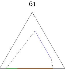
Figure 1.4: Predicted price paths for f = (1, 3, 4, 6) and (i) the agent is rational (blue dashes),(ii)a naive agent experiences cognitive dissonance,δ= 1₂(red), and (iii)a sophisticated agent experiences cognitive dissonanceδ = 1₂(purple)

Some algebra provides

P1_fδ =Eµ(f) +δ (

Eµ(f)−[µ(U)f(uh) +µ(D)f(dh)] )

. (1.4)

When δ = 0the time 1 price corresponds to the rational (and naive) price. As

δ increases Pδ_f decreases, since E_µ(f)−[µ(U)f(uh) +µ(D)f(dl)] < 0. Thus the equity premium at time 1 is given by

−δ(P_f −[µ(U)f(uh) +µ(D)f(dh)]), (1.5)

1.9.2

Response to Information

This section considers an agent satisfying the conditions of the best-case binary dis-tortion and studies his response to information. I find that such an agent deviates from a Bayesian in a rather systematic way. Posterior beliefs are influenced by the agent’s time1choice and are such that the agent always believes his time 1 choice is better than a Bayesian would. It is in this way that the agent exhibits an asym-metric reaction to news. By generally over-valuing his original action it is as if he over-reacts to news that is good for f, while under-reacting to news that is bad for

f.

Research by Easterwood and Nutt [13] suggests that this behavior in fact occurs in financial markets. They study analysts’ forecasts and find that analysts system-atically under-react to negative information and overreact to positive information. Since analysts exhibit both under and overreaction (depending on information), this cannot be due to generic over(under)-reaction to information. For example, a model in which people systematically overreact to information predicts that, after bad news, they should have beliefsmore negativethan the information warrants, whereas the opposite is observed. This phenomena, however, is consistent with the model presented in this paper, under the presumption that an analyst’s decision to cover a stock is seen as an implicit endorsement of the stock.

Definition 1.8. Say that A isgood news for f if f Ax ≻ x for some constant act satisfyingx ∼ f. Similarly, Aisbad news for f ifx≻ f Ax.

sat-isfies Bayes’ rule for all constant scenarios. LetN denote the set of non-constant scenarios.10

Theorem 1.10. If(A, f) ∈ N, thenE_µA,f(u(f))>E_µ|A(u(f)).

Thus an agent that originally chose f will overreact to good news (for f) and under-react to bad news (for f). That is, whenever A is good news for f and f is non-constant on A, the agent overvalues f (relative to a Bayesian). Hence he is willing to pay more for act f, i.e., E_µA,f(u(f)) > E_µ|A(u(f)). Similarly, when A is bad news the agent still overvalues f, and hence under-reacts to the negative information in A.

Additionally, Agrawal and Chen [1] provide evidence that analysts are more op-timistic about firms that have relationships with their employer. This suggests that reference points may have an effect on how people interpret information. The dif-ferential treatment of affiliated and non-affiliated firms is not consistent with any type of non-Bayesian model without reference points, while it is consistent with the model presented here.11

1.9.3

Polarization

While the previous two applications are concerned with the implications of cogni-tive dissonance for a single individual, this section studies the effect of cognicogni-tive dissonance on the distribution of beliefs within a population. In particular, this section shows that whenever two agent take different actions, then even when they observe the same information and have identical prior beliefs they will have differ-ent posterior beliefs.

10_{N ={(A,f)|f(s)≻ f(s˜)for somes, ˜s∈ A}}

11_{It should be acknowledged that both of these explanations require the joint assumption ofbelief}

The seminal experiment on polarization comes from the psychology literature. Lord et al. [45] recruited subjects based on their differing views on the death penalty and presented them with identical essays. Afterwards their views were further apart, even though Bayesian updating predicts they should move closer together. For other explanations of polarization, see [55], [3].

Theorem 1.11. Suppose≿1=≿2 and for all A ∈ Σand f ∈ F,≿1_A,f=≿2_A,f, and

vis strictly increasing. For all A ∈ Σand f,g ∈ F, if(A, f)and(A,g)are such

that for some s,s′ ∈ A, f(s) ≁ g(s) and f(s′) ∼ g(s′), then ≿1_A,f̸=≿2_A,g, hence

µ1

A,f ̸=µ2A,g.

That is, consider two individuals,1and2, and suppose they begin with the same initial beliefsµ. For simplicity, I suppose both agents satisfy the conditions of the proportional distortion for some strictly increasingv. Then whenever the two in-dividuals are in different, non-constant scenarios they will have different posterior beliefs.

..

u

ti

li

ty

i

n

s2

.

utility ins₁ .

f

.

g

..

δ =0

.

δ =1/2

.

δ =1

Figure 1.5: Indifference curves for≿1_A,f and≿2_A,g.

abstain from voting or have not taken an initial stance on an issue will not exhibit polarization, while partisans will exhibit polarization.

However, polarization of beliefs is not simply restricted to the case when agents take different actions. If two agents have differing distortion functions then they may exhibit polarization even after both take the same initial action and observe the same information. Given the abundance of experimental evidence suggesting that an agent’s actions influence how they update their belie