Luo, G. and Yang, S. and Tian, G. and Yuan, C. and Hu, W. and Maybank,
Stephen J. (2014) Learning human actions by combining global dynamics
and local appearance. IEEE Transactions on Pattern Analysis and Machine
Intelligence 36 (12), pp. 2466-2482. ISSN 0162-8828.
Downloaded from:
Usage Guidelines:
Please refer to usage guidelines at
or alternatively
Learning Human Actions by Combining
Global Dynamics and Local Appearance
Guan Luo, Shuang Yang, Guodong Tian, Chunfeng Yuan, Weiming Hu,
Senior
Member, IEEE
, and Stephen J. Maybank,
Fellow, IEEE
Abstract
In this paper, we address the problem of human action recognition through combining global temporal
dynamics and local visual spatio-temporal appearance features. For this purpose, in the global temporal
dimension, we propose to model the motion dynamics with robust linear dynamical systems (LDSs) and use
the model parameters as motion descriptors. Since LDSs live in a non-Euclidean space and the descriptors
are in non-vector form, we propose a shift invariant subspace angles based distance to measure the
similarity between LDSs. In the local visual dimension, we construct curved spatio-temporal cuboids along
the trajectories of densely sampled feature points and describe them using histograms of oriented gradients
(HOG). The distance between motion sequences is computed with the Chi-Squared histogram distance
in the bag-of-words framework. Finally we perform classification using the maximum margin distance
learning method by combining the global dynamic distances and the local visual distances. We evaluate
our approach for action recognition on five short clips datasets, namely Weizmann, KTH, UCF sports,
Hollywood2 and UCF50, as well as three long continuous datasets, namely VIRAT, ADL and CRIM13. We
show competitive results as compared with current state-of-the-art methods.
Index Terms
Action recognition, linear dynamical system, local spatio-temporal feature, non-vector descriptor,
distance learning.
F
1
I
NTRODUCTIONAnalysis of human activities concerns detecting, tracking, recognizing and understanding human
movements from image sequences. Among these problems, human action recognition is one of the
most active research areas and has attracted much research interest over the past couple of decades.
The surveys by Turaga et al. [1] and Poppe [2] provide a broad overview of numerous approaches
for analyzing human motion sequences in videos. In terms of the motion sequence representation,
previous work can be roughly classified into appearance-based methods and motion-based methods.
Appearance-based methods usually characterize the motion sequence with various local [3], [4], [5],
• G. Luo, S. Yang, G. Tian, C. Yuan and W. Hu are with the National Laboratory of Pattern Recognition, Institute of Automation, Chinese Academy of Sciences, No. 95, Zhongguancun East Road, PO Box 2728, Beijing, 100190, P.R. China.
E-mail:{gluo, syang, gdtian, cfyuan, wmhu}@nlpr.ia.ac.cn.
[6] or global [7], [8], [9], [10] visual features extracted from raw video data. For example, Niebleset
al.[6] use a bag-of-words model to represent human actions. The bag-of-words model is learned by
extracting and clustering local spatio-temporal interest points. The major problem in these methods is
that they discard the temporal information inherent to actions and thus fail to capture the temporal
dynamics of human activities. Motion-based methods generally model the motion sequence with
temporal state-space models [11], [12], [13], [14] and view the human action recognition as a temporal
classification problem. For example, Yamatoet al.[11] propose to recognize tennis shots by modeling
a sequence of grid-based silhouette features as outputs of class-specific HMMs. However, these
methods are of comparatively high complexity and require detailed statistical modeling and parameter
learning. They also do not model the motion dynamics in an explicit way.
It is known that appearance and dynamics are two important cues for human action recognition.
However, the capture of both global temporal dynamics and local visual appearance features of
action sequences has always been a challenging task, and few attempts have been made to explore it.
Mikolajczyk and Uemura [15] extract both local appearance features (i.e. MSER, Harris-Laplace and
Hessian-Laplace) and local motion features (i.e. dominant motion compensation) to jointly represent
human actions. These appearance-motion features are clustered to form many vocabulary trees.
Votes for action categories are given by matching features extracted from query frames to the trees.
Artizzuet al.[16] combine weak trajectory features with popular spatio-temporal features to recognize
long-time continuous social behaviors. Weak trajectory features, such as agent distance, movement
direction, velocities and accelerations are computed based on the tracked agent positions. Finally,
temporal context features are adopted to improve the classification performance. They conclude that
the combination of appearance and motion features outperforms their use separately, and suggest that
behavior understanding should be based on such heterogeneous features. Since these methods can
be regarded as feature-level combinations of local appearance and motion features, Wanget al. [10]
use a multi-channel approach to fuse different distance matrices computed with HOG (histograms
of oriented gradients), HOF (histograms of optical flow) and MBH (motion boundary histograms).
They calculate theχ2 distance matrix separately for each channel, and then sum them up, weighted
by their respective mean values, to form the final RBF-χ2 kernel. This method can be regarded as a
decision-level combination. Our approach is in part similar to that of Wanget al. [10], but different
in two aspects. First, we compute the robust LDS over the whole action sequence to describe the
global dynamics. In this way, we expect to capture the global temporal evolution of action sequences,
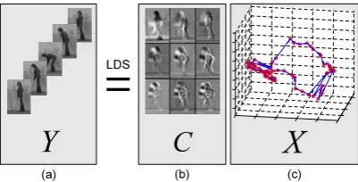
even when this can not be achieved with local motion features. Fig. 1 gives an example of how a
robust LDS captures the temporal dynamics of action sequences. With robust LDS, an action sequence
is decomposed into subspace components and state sequence, in which the latter represents the
temporal variations. Second, we combine the global dynamics and local appearance in a maximum
margin distance learning framework. The combination weights are learned, to balance the importance
of motion and appearance features, such that the action classes are maximally separated. In addition,
we point out that our combination framework can be easily extended to three or more heterogeneous
=
<
&
;
(a) (b) (c)
[image:4.595.197.398.71.173.2]LDS
Fig. 1. This example illustrates the robust LDS representation of action sequences. (a) A video
sequence Y is decomposed into two parts with robust LDS. (b) The subspace components C show
the principal action appearance. (c) The state sequenceX illustrates the motion dynamics over time.
1.1 Motivation and Overview
LDS and its extensions [17], [18], [19], [20] have long been studied for human motion analysis. They
demonstrate superiority over common HMMs on classification task, but generally require complex
Bayesian modeling and inference. Recent advances in system identification theory for learning LDS
parameters [21], [22] and similarity measures between LDSs [23], [24], [25], [26] have made LDS
successful for classification of high-dimensional time-series data in the field of dynamic texture [27],
[28]. This poses us a new way to model and compare action sequence dynamics. By modeling the
temporal variations with LDS, system theoretic methods specifically consider the global dynamics of
action sequences. The similarity between two LDSs is directly measured with a distance or kernel
metric defined on the LDS space. Considering that sequence similarity based on local appearance
features is commonly computed with a distance metric defined on the histogram space, this inspires
us to combine the global dynamics and local appearance features in a unified framework.
Following this idea, our study in this paper aims to combine global dynamics, which are described
with robust LDS, and local appearance, which is represented by dense curved spatio-temporal cuboids
[10], for human action recognition in a maximum margin distance learning framework. The main
motivation behind this method is to model the distance between two sequences as a weighted sum
of the respective distances obtained from global dynamics and local appearance features. Recognition
is carried out by learning the weights in a way that maximizes the class discrimination. By this
means, LDSs and cuboids are complementary in describing action sequences by capturing both motion
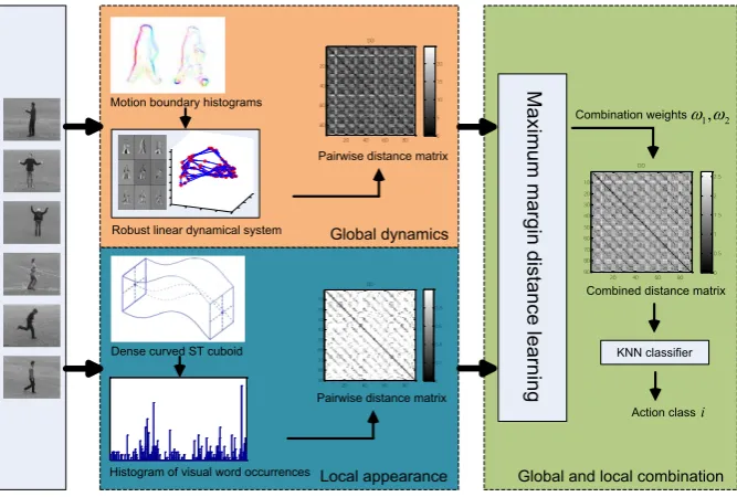
dynamics and visual gradients. Fig. 2 shows the system diagram of our proposed method.
Furthermore, we find that stability is a crucial property for dynamical systems, whereas it is
generally omitted by most of previous work [9], [26], [27], [29], though it has been intensively
studied in the system identification literature [21], [30], [31]. This motivates us to introduce an efficient
optimization method to learn robust LDS. We also develop a shift invariant distance metric based
on the subspace angles distance [24]. We demonstrate that our distance metric is insensitive to the
starting frame of action sequences, and thus outperforms the traditional metrics in recognition rate.
1.2 Contributions
Global dynamics
Local appearance
Robust linear dynamical system
DD
20 40 60 80 20 40 60 80 0 5 10 15 20
Pairwise distance matrix
DD
20 40 60 80 10 20 30 40 50 60 70 80 90 0 0.2 0.4 0.6 0.8
Pairwise distance matrix Motion boundary histograms
Global and local combination
Maxi m u m marg in d istanc e lea rn in g DD
20 40 60 80 10 20 30 40 50 60 70 80 90 0 0.5 1 1.5 2 2.5
Combined distance matrix
Dense curved ST cuboid
Histogram of visual word occurrences
Action classi
1, 2 w w Combination weights
[image:5.595.131.465.71.296.2]KNN classifier
Fig. 2. System diagram of the proposed method. For global dynamics, MBH is extracted in each frame
and robust LDS is learned based on MBH sequences. Distance matrix is computed using a shift invariant
distance metric. For local appearance, HOG is calculated for each dense curved spatio-temporal cuboid.
Occurrence histogram is built in the bag-of-words framework and Chi-Squared distance is computed to
measure the pairwise distance. Finally, these two distance matrices are combined in a maximum margin
distance learning framework. Action classification is achieved by using a KNN classifier.
• We propose to combine LDSs and cuboids for human action recognition in a maximum margin
distance learning framework. The LDSs and cuboids capture not only local visual information of
action appearance, but also global dynamic information of human movements. To the best of our
knowledge, there is no other work which considers this approach to recognize human actions.
• We introduce a simple yet efficient robust LDS learning algorithm to describe action sequence
dynamics. A suboptimal solution is achieved by iteratively checking stability criteria and
gen-erating new constraints. The process is repeated until it finds a stable solution. We show that
sequences evolved with robust LDS share the same dynamic characteristics as the training data.
This is essential for our proposed shift invariant distance metric.
• We develop a shift invariant distance metric which is robust to the initial conditions of the LDS,
thus is insensitive to the starting frame of the action sequences. This is based on the considerations
that the classification of an action sequence should be independent of the frame that it begins
with. The state-of-the-art methods do not achieve this purpose.
• We carry out extensive experiments on eight public datasets. We evaluate the robust LDS on the
selection of model parameters, and compare to the traditional LDS as well as three other temporal
methods, namely MEMM [32], CRF [13] and switching LDS [19] to quantify the improvement in
recognition rates. Furthermore, we evaluate the performance achieved with LDSs and cuboids
alone, as well as the combination of these two components. We compare to current state-of-the-art
1.3 Organization
Section 2 reviews related work on appearance-based and motion-based methods for human action
recognition. Section 3 firstly introduces LDS and describes how LDS parameters are learned in the
literature. Then a robust LDS learning algorithm is introduced and analyzed in detail. Finally a shift
invariant distance metric is proposed to measure the distance between LDSs. Section 4 briefly outlines
the recognition pipeline of bag-of-words and shows how dense curved spatio-temporal cuboids are
constructed and described in our work. Section 5 presents the maximum margin distance learning
algorithm and illustrates how LDSs-based distance and cuboids-based distance are combined for
human action recognition. Section 6 shows the experimental results including comparisons with
competing methods for learning human actions. Section 7 gives the conclusions plus some ideas
for further work.
2
R
ELATEDW
ORKIn Section 1, we briefly reviewed the work on motion representation in order to make clear the
motivation for this paper. In this section, we review in detail the human action recognition methods
in order to put our work into context. For clarity, we divide the existing work into two categories:
appearance-based methods and motion-based methods.
2.1 Appearance-based Methods
Appearance-based methods usually extract local or global visual features from video data for human
motion analysis. Local approaches involve detecting and describing spatio-temporal interest points
to represent human activity. Laptev [3] extends the Harris detector to video in both spatial and
temporal domains. However, this detector only finds a small number of stable interest points, which
are usually insufficient for motion analysis and classification. Doll´aret al. [4] improve the 3D Harris
detector by applying Gabor filtering in the spatial and temporal dimensions separately. By choosing
proper spatial and temporal scales, the detector can yield a large number of cuboids. Oikonomopoulos
et al.[33] present a saliency detector based on a computed entropy of each cuboid. The cuboids with
the local maximum entropy value are selected as salient points. Willems et al. [34] identify saliency
with the determinant of a 3D Hessian matrix, which can be calculated efficiently using the integral
videos. Seo and Milanfar [35] use space-time local steering kernels to capture the underlying geometric
structures of action sequences. They show good performance with only one training example. Mathe
and Sminchisescu [36] propose saliency map prediction models, which are learned from human eye
fixated regions for action recognition. They illustrate comparable results to those obtained using dense
sampling with sparse uniform sampling. These methods treat space and time in the same manner.
However, action videos normally show different characteristics in space and time. It is therefore
more suitable to handle space and time differently, rather than to treat them in a joint 3D space.
Wong and Cipolla [37] detect interest points separately on subspace images and coefficient vectors by
address this problem by designing a novel anisotropic filter in the temporal dimension and applying
an isotropic Gaussian filter in the spatial domain. Wang et al.[10] handle space and time differently
by tracking densely sampled interest points through video sequences. The resulting trajectories and
the aligned space-time volumes are used to represent the videos. To describe spatio-temporal points,
feature descriptors are calculated in the neighborhoods of selected points using image measurements
such as spatial or spatio-temporal gradients. Sch ¨uldt et al. [39] calculate normalized derivatives in
both space and time. Doll´ar et al. [4] experiment with image brightness, gradient and optical flow
information. Scovanner et al. [5] extend the popular SIFT descriptor [40] to the space-time domain
and develop a 3D SIFT. Willems et al. [34] generalize the SURF descriptor [41] by computing a
weighted sum of space-time Haar-wavelets in grid cells. Wanget al.[10] combine local HOG, HOF and
MBH descriptors to achieve state-of-the-art results. Local methods have shown many encouraging
results because of their reliability in the presence of background noise, geometric variation and
occlusion. However, there exists a limitation for these approaches in that they do not incorporate
global information and ignore the temporal variations of human actions.
Global approaches generally use global features such as optical flow and silhouettes to capture
the motion information in action sequences. Efros et al. [7] use blurred optical flow histograms to
match actions in sport videos. Ali and Shah [42] derive kinematic features from optical flows. PCA
is applied to determine the dominant kinematic modes. Action recognition is performed by using
multiple instance learning approach. Wanget al. [10] introduce a descriptor by tracking dense points
based on the optical flow field. Instead of extracting optical flow, the silhouette of a person in the
image is used for recognition. Bobick and Davis [43] extract silhouettes and use temporal templates
for the representation and recognition of aerobics actions. Wang and Suter [44] project silhouette
sequences into a low-dimensional subspace to characterize the space-time properties of human actions.
However, optical flow and silhouettes are very sensitive to background noise, viewpoint variation as
well as occlusions. To address these issues, Tranet al.[8] divide the silhouettes and optical flow fields
into rectangular grids. A motion descriptor is developed by combining both horizontal and vertical
components of optical flow as well as the silhouette of person. Gorelicket al.[45] stack silhouettes over
time to form a space-time volume. Local space-time saliency and orientation features are derived by
solving a Poisson equation. Global approaches perform well because they encode much of the motion
information. However, they depend strongly on the recording conditions, in order to realize accurate
localization, background subtraction or tracking. In addition, these approaches also do not model the
temporal dynamics of global features.
2.2 Motion-based Methods
Motion-based methods usually model the action sequences with temporal state-space methods such
as HMMs, conditional random fields (CRFs) or dynamical systems. Brandet al.[12] propose a coupled
HMM to represent the interaction between subjects. Cailletteet al.[46] use a variable length Markov
model (VLMM) to describe the observations and 3D poses for each action. Hongeng and Nevatia [47]
resulting in a hidden semi-Markov model (semi-HMM) to achieve event detection. HMMs are efficient
for modeling time series data. However, their application is restricted due to the assumptions of
conditionally independent observations and Markov property for the sequence of hidden states. CRFs,
on the other hand, avoid these two assumptions and allow non-local dependencies between states and
observations. Sminchisescuet al.[13] use CRFs for human motion recognition. They show that CRFs
outperform both HMMs and maximum entropy Markov model (MEMM) when a longer observation
history is taken into account. Vail et al. [14] compare CRFs and HMMs in detail and conclude that
CRFs perform as well as or better than HMMs. Natarajan and Nevatia [48] propose a two-layer
model and use CRFs to encode actions and viewpoint-specific poses. However, despite that HMMs
and CRFs model action sequence as a time-varying series, they do not model the motion dynamics
in an explicit way.
Dynamical system methods capture the temporal variations by decoupling the action sequence
into subspace poses and latent dynamics. Bregler [17] proposes a multi-level framework for learning
and recognizing human dynamics. LDSs are used to describe the mid-level simple movements, while
HMMs are learned to represent the high level complex behaviors. Blake et al. [18] represent the
multi-class motion sequence with a mixed auto-regressive process. Model parameters are learned
by combining the expectation maximization (EM) with the Condensation algorithm. Pavlovic and
Rehg [19] model the nonlinear dynamics in human motion with switching LDSs, whereas model
learning and inference are based on a variational technique. Turagaet al.[20] model an action sequence
as a cascade of LDSs. They simultaneously segment the sequence in the temporal dimension and learn
an LDS for each segment. Wanget al.[49] explore the nonlinearity of motion sequences with Gaussian
process dynamical models. Model parameters are marginalized out in closed form rather than being
estimated. This results in a nonparametric model for dynamical systems. Though dynamical system
approaches are powerful for describing the motion sequence dynamics, they usually require detailed
statistical modeling and parameter learning. In addition, exact inference is generally intractable and
approximation methods have to be developed.
Recent work reported in the system identification literature makes the comparison between
dy-namical systems straightforward by directly defining distance or kernel metrics in the model space.
Martin [23] defines a metric for stable ARMA models based on a comparison of their cepstrum
coefficients. De Cock and De Moor [24] extend the concept and propose to compare stable ARMA
models by using the subspace angles between two systems. Chan and Vasconcelos [25] derive a
probabilistic kernel based on Kullback-Leibler divergence and use it for dynamic texture classification.
Vishwanathanet al.[26] present a generic similarity metric for dynamic scene analysis based on the
Binet-Cauchy theorem. Since most of the work is designed for dynamic textures, few attempts have
been made for human motion recognition. Bissaccoet al. [50] extend the work in [26] and define a
novel kernel-based distance on LDSs for human gait recognition. Chaudhry et al. [9] encode each
frame of an action sequence using a histogram of oriented optical flow (HOOF) and employ
Binet-Cauchy kernels [26] to describe the HOOF sequence. In this paper, we argue that previous work for
[
[
\
\
W W[
$
&
\
Fig. 3. Graphical model representation of LDS. The grey elementyidesignates the observable feature
or image. The white element xi represents the unseen or latent state variable. The parameter A
indicates the dynamic matrix, while parameterCindicates the subspace mapping matrix.
to the initial conditions. To address these issues, we introduce a robust LDS learning algorithm and
develop a shift invariant distance metric. We demonstrate encouraging recognition results on both
short clips datasets and long continuous datasets.
3
R
ECOGNITION WITHR
OBUSTLDS
SDynamical system methods have been studied extensively in fields ranging from control
engineer-ing to visual process. Among all the methods, LDS is used broadly because of its simplicity and
efficiency. For instance, many dynamic texture recognition methods represent the texture’s temporal
variation as an LDS [27], [28]. From the graphical model’s perspective, as illustrated in Fig. 3, LDS
is indeed a generative state-space model with Gaussian observations and Markov states. For human
action sequences, many inherent nonlinearities such as phase transition, turbulence and delay can be
eliminated by choosing proper coordinates or mapping into high-dimensional spaces [50]. Therefore
in this paper, we focus on how to model the human motion dynamics with LDS.
3.1 Linear Dynamical Systems
LetA∈Rn×ndenote the system dynamic matrix, andC∈Rp×ndenote the subspace mapping matrix.
Here pand n are the dimensions of the observation space and the state space, respectively. Then a
stationary LDS can be represented by the parameter tupleM= (A, C)and evolves in time according
to the following equations
xt+1=Axt+vt
yt=Cxt+wt
(1)
wherext∈Rnis the state or latent variable,yt∈Rpis the observed random variable or feature,vtand
wt are the system noise and observation noise, respectively. If we assume the noises are zero-mean
i.i.d Gaussian processes, then we have vt∼ N(0, Q) andwt∼ N(0, R). HereQand R are covariant
matrices of multivariate Gaussian distributions.
In (1) the hidden state is modeled as a first-order Gauss-Markov process, wherext+1is determined
by the previous statext. The outputytdepends linearly on the current statext. Given a video sequence
y1:τ, learning the intrinsic dynamics amounts to identifying the model parameterM. This is a typical
(a) (b) (c) (d) (e)
(f) (g) (h) (i) (j)
Fig. 4. State sequences (n= 3) of 10 different actions performed by one subject from the Weizmann
dataset. (a) bend, (b) jack, (c) jump, (d) pjump, (e) run, (f) side, (g) skip, (h) walk, (i) wave1, (j) wave2.
Let column matrixY1:τ= [y1, y2, ..., yτ]andX1:τ= [x1, x2, ..., xτ]represent the observation sequence and state sequence, respectively. In order to get a closed form estimate of the model parameter
M, the observation matrix is firstly decomposed with the singular value decomposition (SVD), i.e.
Y1:τ =UΣVT, whereU,V are orthogonal andΣis a rectangular diagonal matrix with non-negative
real numbers on the leading diagonal. An estimate of the subspace mapping matrix and the underlying
state sequence is obtained by setting
ˆ
C=U, Xˆ1:τ = ΣVT (2)
The model dimensionnis determined by retaining the singular values which exceed a given threshold.
Then the least squares estimation ofAis
ˆ
A= arg min
A ∥A
ˆ
X1:τ−1−Xˆ2:τ∥F2 = ˆX2:τXˆ1:+τ−1 (3)
where∥ · ∥F denotes the Frobenius norm and+ denotes the Moore-Penrose inverse. Given the above
estimates ofAˆ andCˆ, the covariance matricesQˆ and Rˆ can be estimated directly from residuals.
According to Eq. (2), LDS implicitly models the observationY1:τ with a subspace mapping matrix
C and its corresponding coefficients X1:τ. In human action recognition task, as shown in Fig. 1, the
subspace matrix C describes the action components, while matrix A, which is derived from X1:τ,
represents the motion dynamics. Thus we can use M = (A, C) to represent the motion sequence
descriptor. Such a descriptor captures both the dynamics and the embedding components of an action
sequence, and is thus very different from the local spatio-temporal gradient descriptors. In Fig. 4, we
show the state trajectories of ten action classes from the Weizmann dataset, from which we can see
that the trajectories behave very differently among different actions. This makes it possible to classify
and recognize them by exploring the dynamics.
However, there exist two problems when using M as the descriptor. The first one is that the
traditional LDS solvers ignore the stability of dynamical systems. This may result in a degenerate
LDS model. The second one is that the descriptor is represented using the tupleM= (A, C), which
lives in a non-Euclidean space and is in non-vector form. There is no straightforward way to compute
the non-vector descriptor distance in a non-Euclidean space, let alone find distance metrics which are
)UDPH
#15
#30
#45 #58
#73 #87
Fig. 5. State sequence X1:τ learned with a jumping jack video from the Weizmann dataset. The
sequence has total 89 frames with three cycles. A robust LDS is learned with the state dimension
n= 3. The three state components are figured as blue, red and green curves, respectively. The sample
images corresponding to the key periodic frames are also demonstrated.
3.2 Learning Robust LDS
Stability is a very important property for LDSs and it has been intensively studied in the system
identification literature. An unstable LDS may fail to generate long sequences which share the same
characteristics as the original data. However, we find that most of the previous work [9], [26], [27], [29]
has omitted this problem. This may cause the failure of distance computations between descriptors
because the distance or kernel metrics for dynamical systems are mostly defined on stable models [23],
[24], [26]. We show in Section 3.3 that generating consistent data is critical for our proposed shift
invariant distance metric.
Let{λ1, λ2, ..., λn}denote the eigenvalues of dynamic matrix Ain decreasing order of magnitude.
The system spectral radius is defined asρ(A)≡ |λ1|. An LDS is called stable if and only ifρ(A)≤1.
Ifρ(A) = 1, the system is said to be marginally stable. Marginally stable systems are very useful as they generate sustained oscillations in the output, which in our case describes the periodic patterns in
motion sequences. In Fig. 5, we show an example of a periodic action sequence from the Weizmann
dataset. By learning the robust LDS, we obtain a state sequence which varies periodically with
the observation sequence. This means that robust LDS captures the intrinsic dynamics of cycle
movements. However, traditional LDS learning methods such as (3) do not enforce this stability
criterion. This may cause the solution to be unstable even if the true system is stable.
Some robust techniques in the literature have been developed based on searching through a full
feasible set of dynamic matrices [31] or on improving the least squares objective function with
regularization terms [30]. The N4SID method [21] achieves optimal solutions in the sense of maximum
likelihood. However, it is computationally expensive to obtain the optimal solutions for these methods.
In our case of human action recognition, we do not require precisely optimal results. We prefer
an efficient approximation solution, provided it satisfies the stability criterion. Here we introduce a
constraint generation method [51], which achieves a stable result efficiently by iteratively checking
the stability criterion and generating new constraints. The main idea of this approach lies in
formu-lating the least squares problem in (3) as a quadratic program with linear constraints. These linear
constraints, which are initially void, are inferred iteratively using the stability criterion. The optimal
(a) (b)
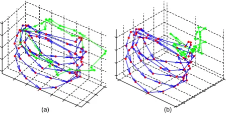
Fig. 6. Generation comparison between robust LDS and traditional LDS. The red trajectories in (a)
and (b) illustrate the state sequences learned with robust LDS (a), and traditional LDS (b) respectively,
using the same walking video in each case. The green trajectories are generated by evolving the red
sequences 28 steps ahead with their respective LDS, from which we see that the unstable LDS (b)
cannot generate new data consistent with the given data.
The least squares problem in (3) can be reformulated by expanding the right hand side as
ˆ
A= arg min
a {a
TP a−2qTa+r} (4)
where a=vec(A),q =vec( ˆX1:τ−1Xˆ2:Tτ),P =In⊗( ˆX1:τ−1Xˆ1:Tτ−1), andr=tr( ˆX2:TτXˆ2:τ). Herevec(·) is a linear operator which flattens the matrix to vector in column order.
The linear constraints are obtained by decomposingAˆusing SVD Σ = ˆˆ UTAˆVˆ and inferring as
˜
λ1= ˜uT1Aˆv˜1=tr(˜v1u˜T1Aˆ) =g
Tˆa≤1
(5)
whereg=vec(˜u1v˜1T),ˆa=vec( ˆA),u˜1and v˜1 are the singular vectors corresponding to ˜λ1.
Therefore, the quadratic program can be written as
minimize aTP a−2qTa+r
subject to gTa≤1 (6)
This quadratic program is repeatedly invoked until the stability criterion is satisfied. At each
iteration, a new linear constraint is calculated with (5). Considering that g depends on a, it is
therefore an approximation solution to holdg fixed. In Fig. 6, we compare the generation capability
between robust LDS and traditional LDS, from which we can see that the robust LDS generates new
data illustrating the same dynamic characteristics as the training sequence, while the traditional one
generates cluttered data which are very different from the original data.
3.3 Shift Invariant Distance Metric for LDS
Given an action sequence, we use the robust LDS model parameterM= (A, C)as a motion sequence
descriptor, with the dynamic matrix A ∈ GL(n), where GL(n) is the group of all n×n invertible
matrices, and with the mapping matrixC∈ST(p, n), where ST(p, n)is the Stiefel manifold. Since the
model space has a non-Euclidean structure and the descriptor is in non-vector form, this naturally
raises the issue of how to measure the similarity between two descriptors. In one of the first papers
their cepstrum coefficients. De Cock and De Moor [24] improve Martin’s work by using the subspace
angles between two LDSs. The subspace angles are defined as the principal angles between the
column spaces of infinite observability matricesO∞(Mi) = [CiT (CiAi)T (CiA2i)T . . .]T ∈R∞×n
fori= 1,2.
LetM1= (A1, C1)and M2= (A2, C2)denote the two motion sequence descriptors. The
computa-tion of subspace angles is obtained by solving the Lyapunov equacomputa-tion
Q=ATQA+CTC (7)
forQ, where Q=
Q11 Q12
Q21 Q22
∈R2n×2n,A=
A1 0
0 A2
∈R2n×2n,C= (C
1 C2)∈Rp×2n.
The solution of (7) is guaranteed to exist whenM1andM2are stable. The cosines of the subspace
anglescos2θ
iare calculated as eigenvalues of matrixQ−111Q12Q−221Q21, whereQkl =O∞(Mk)TO∞(Ml) fork, l= 1,2.
The subspace angles distance is defined as
dLDS(M1,M2)2=−log
n
∏
i=1
cos2θi (8)
Vishwanathanet al.[26] present a generic kernel metric for dynamical systems based on the
Binet-Cauchy Theorem. For two LDSsM1 and M2 which evolve with independent noise realization, the
Binet-Cauchy kernel is computed by firstly solving a Sylvester equation
S=e−λAT1SA2+C1TC2 (9)
forS, where e−λ is an exponential discounting term withλ >0.
The above Sylvester equation can be solved efficiently by rewriting it as
vec(S) =vec(e−λA1TSA2) +vec(C1TC2)
= (AT2 ⊗e−
λ
AT1)vec(S) +vec(C
T
1C2)
(10)
Thus we have
vec(S) = (I−AT2 ⊗e−λAT1)−1vec(C1TC2) (11)
After reshaping vec(S)into matrixS, the Binet-Cauchy kernel is defined as
kLDS(M1,M2) =x1(0)TSx2(0) (12)
on condition thate−λ∥A
1∥ ∥A2∥<1. Herex1(0),x2(0)are the initial states ofM1andM2, respectively.
From (12), we see that the Binet-Cauchy kernel depends directly on the initial conditions.
Exper-iments also show that subspace angles distances and Binet-Cauchy kernels vary greatly when two
sequences differ by only a temporal shift (see Fig. 7, blue square). In our case of human action
recognition, we require a distance measure that is insensitive to the initial state. In other words, two
walking sequences should be classified into the same category no matter what frame they begin with.
Hence we develop an offset alignment strategy by evolving each sequence for a number of steps such
that the distance between them is minimized. That is
d(M1,M2) = min
τ1,τ2∈N
or
k(M1,M2) = max
τ1,τ2∈N
kLDS(M1(τ1),M2(τ2)) (14)
where M(τ)denotes the model parameter of evolved sequence which is generated by shifting the
original sequence τ steps ahead. We notice that a robust LDS model must be learned to ensure that
the evolved sequences have the same characteristics as the original sequence. This is why model
stability is especially important for our algorithm.
It is unfortunate that there is no an explicit way to obtain the solutions of (13) and (14). However
in many applications, the periods of most motion patterns are short. Thus we can solve this problem
by searching through all the combinations ofτ1 andτ2 exhaustively. IfT is an upper bound for the
shift, then the complexity of this problem isO(T2). In practice, we can speed up the computation by
caching both the originalM and its T shifted versions M(τ) forτ = 1, ...,T. The detail of the shift
invariant distance metric algorithm is presented in Algorithm 1.
Algorithm 1 Shift Invariant Distance Metric Algorithm
Input: Given two sequencesY1 andY2;
1: Learn robust LDSM1= (A1, C1)andM2= (A2, C2)according to (6);
2: forτ=1:T do
3: %Subroutine to evolveY1 andY2 forτ steps respectively
4: Initializex0 as the last state of the learned state sequence;
5: fori= 0 :τ−1do
6: xi+1=A∗xi+mvnrnd(0, Q)
7: yi+1=C∗xi+1+mvnrnd(0, R)
8: end for
9: Learn robust LDSM1(τ)andM2(τ)based on evolved sequencesY1(τ)andY2(τ);
10: end for
11: Compute all pairwise distance metrics betweenM1(τ1)andM2(τ2)according to (8) or (12);
12: Compute the shift invariant distance metric based on (13) or (14);
Output: Shift invariant distance metricd(M1,M2)ork(M1,M2);
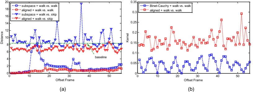
We show in Fig. 7 that our shift invariant distance metric outperforms the standard metrics in two
aspects. First, the aligned distance/kernel exhibits a better similarity measure than the original
sub-space angles distance and Binet-Cauchy kernel. This results in better recognition results as illustrated
in Fig. 9a. Second, the aligned distance/kernel is more stable with respect to frame offset, whereas
the subspace angles distance shows sudden changes in some conditions and the Binet-Cauchy kernel
exhibits periodic variations with the periodic change of the starting frame. In addition, in Fig. 7a, we
compare the aligned distance and subspace angles distance between different action classes, i.e. walk
vs. skip. We see that although the aligned distances between different classes are reduced (red triangle
vs. blue triangle), the separation between the intra-class and inter-class distances (red square vs. red
triangle) is very clear. On the other hand, this separation is not so clear for the original subspace
angles distances (blue square vs. blue triangle). Specifically, we choose the maximum walk vs. walk
D
0 10 20 30 40 50
0 2 4 6 8 10 12 14 16 18 20
Offset Frame
D
is
ta
n
c
e
subspace + walk vs. walk aligned + walk vs. walk subspace + walk vs. skip aligned + walk vs. skip
baseline
E
0 10 20 30 40 50
0 0.05 0.1 0.15 0.2 0.25 0.3 0.35
Ke
rn
e
l
[image:15.595.95.505.72.220.2]Offset Frame Binet-Cauchy + walk vs. walk aligned + walk vs. walk
Fig. 7. Comparison of subspace versus aligned distances (a), and Binet-Cauchy versus aligned
kernels (b). The ’square’ distances/kernels are computed between a model learned from a walking
sequence and the set of models learned from the same sequences with different starting frames. The
’triangle’ distances are computed in the same way between the walking sequence and shifted skipping
sequences. The baseline is chosen as the maximum walk vs. walk subspace angles distance. The
’blue’ distances between different classes, say walk vs. skip, which are below the baseline may cause
misclassification.
which are below the baseline may cause misclassification.
4
R
ECOGNITION WITHC
URVEDS
PATIO-T
EMPORALC
UBOIDSLocal spatio-temporal appearance features are successful for many visual tasks. They capture
char-acteristic shape, texture and local motion in video sequences. These charchar-acteristics are good
com-plements to the global dynamics. In Section 2, we reviewed the state-of-the-art local approaches. In
this paper, we use the dense curved spatio-temporal cuboids [10] as local appearance features and
describe them with HOG descriptors. This is based on the consideration that the dense sampling
method has proved its effectiveness and achieves state-of-the-art recognition results on a wide range
of human action datasets.
Given an action sequence, we first densely sample interest points on a grid in each frame. Then
these points are tracked based on the dense optical flow field to form dense trajectories. The curved
spatio-temporal cuboids are constructed as the local space-time volumes along the trajectories. The
size of the cuboid is N ∗N pixels and L frames long. Since the trajectories are curves in
space-time domain, we call these space-space-time volumes ’curved cuboids’, to differentiate from the traditional
’straight cuboids’ [4].
To describe the curved spatio-temporal cuboids, we subdivide each cuboid into a spatio-temporal
grid of size Nσ∗Nσ∗Nτ. We compute HOG in each cell of the grid to create a sub-histogram, and
concatenate all the sub-histograms to obtain the final descriptor.
Once we obtain all the HOG descriptors on the dataset, we quantize them into visual words byk
-means clustering. Then we represent each sequence as the frequency histogram over the visual words.
(X2) distance
dST C(H1, H2) = 1 2
∑
i
(H1(i)−H2(i))2
H1(i) +H2(i)
(15)
5
C
OMBININGLDS
S ANDC
UBOIDS BYM
AXIMUMM
ARGIND
ISTANCEL
EARNINGIn this section, we combine LDSs-based distance dLDS and cuboids-based distance dST C in a
maxi-mum margin learning framework. The final distance between two sequences is computed as a linear
combination ofdLDSanddST C. The weights for the linear combination are learned with the maximum
margin distance learning algorithm [29] in such a way that the action classes are maximally separated.
Let a set of training sequences be given with class labels inc={1, ..., N}and letli be the label of
sequencei. The global dynamic distance from sequencej toi is denoted asdLDS(ij), and the local
appearance distance isdST C(ij). Then the combined distance from sequence j toi is defined as
D(ij) =ω1(li)dLDS(ij) +ω2(li)dST C(ij) =ω(li)Td(ij) (16)
whereω(li)is the vector of class dependent weights that characterize the corresponding distance for
classli. Similarly, we define the class independent distance by dropping the class labelli from (16).
In order to maximally separate the classes of sequences, we define a representative set R(i) of
sequenceias itsk-nearest neighbors within its class, and a comparative setC(i)as all other sequences
outside its class. We assume that a sequence is closer to the sequences in its representative set than
to those in its comparative set. That is, for all i̸=j, j ∈ R(i) and k ∈ C(i), we have the following
distance constraints
D(ij)≤D(ik)⇒ω(li)T △d(i)≥0 (17)
where △d(i) =d(ik)−d(ij) is the distance difference vector from the sequence in the comparative
set to the sequence in the representative set.
In the class dependent case, the total number of such constraints in classcisL=∑l
i=c|R(i)||C(i)|.
By embedding these constraints in a maximum margin framework,ω(c)can be found by minimizing
min ω(c)
λ
2∥ω(c)∥ 2+ 1
L
L
∑
i=1
max(0,1−ω(c)T △d(i)) (18)
whereλis the regularization parameter. This problem is similar to the problem of learning a support
vector machine (SVM). It can be efficiently solved with the Pegasos algorithm [52].
After obtainingω(c)for each class, a test sequence is classified as the class which satisfies the most
number of distance constraints generated by the test sequence.
6
E
XPERIMENTSTo evaluate the performance of our proposed method for human action recognition, we carry out
detailed experiments on the state-of-the-art datasets. We first briefly introduce the experimental setup,
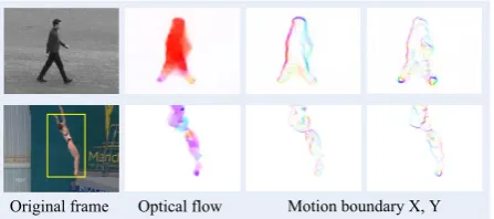
Optical flow Motion boundary X, Y Original frame
Fig. 8. Illustration of raw, optical flow and MBH (x, y) images of two action sequences from the KTH
dataset (top) and the UCF sports dataset (bottom), respectively. For the optical flow and MBH images,
gradient/flow orientation is indicated by color (hue) and magnitude by saturation.
6.1 Experimental Setup
6.1.1 Feature Extraction
To compute robust LDS, we extract sequential features from all the videos. Our proposed method can
be used with different types of features, including even raw pixels, provided that the features form
a time series. Silhouettes or shape features [44] are useful, but they are difficult to obtain in
uncon-strained environments. In this paper, we use the motion boundary histograms [53] to characterize the
action profile. The MBH encodes the relative motion between pixels by computing gradients of thex
andy optical flow components separately. It suppresses most of the camera motion and background
texture, and thus highlights the foreground subject. Some examples are illustrated in Fig. 8.
As suggested in [53], we resize the sequences into 64×128 pixels. The MBH is computed by
quantizing the orientations into9bins with2×2blocks of8×8pixel cells. To improve the performance,
block overlap (0.5) is also incorporated. Thus we obtain a total of 7×15 blocks, where each block
is described by a4×9 histogram. The final histogram size is3780 for bothxand y components of
MBH (i.e.,7×15×36).
For local appearance, we take the same parameters as used in [10]. The size of the curved cuboid is
32×32pixels and15frames long. Each cuboid is divided into2×2×3cells, and each cell is described
with a8-bin histogram. Thus the final HOG descriptor size for each curved cuboid is96. We randomly
choose100,000training cuboids to form a codebook of4,000visual words withk-means. The resulting
frequency histograms over the visual words are used as sequences representation.
6.1.2 Robust LDS
There are two parameters related with robust LDS: model dimensionnand upper bound of temporal
shiftT. We evaluate the performance for different values of these parameters in Section 6.3.1 and 6.3.2.
We choosen = 3 and T = 16as default parameters in our experiments by considering the balance
of recognition performance and computational cost.
6.1.3 Baseline Temporal Models
To quantify the improvement obtained with the robust LDS, we compare to the traditional LDS as well
presented in the following. For all these models, we use the same MBH sequences as input features.
We implement the traditional LDS via least squares estimation according to Eq. (2) and (3). We
use the same setup as for the robust LDS, except that the stability criterion is not incorporated. We
compute LDS with model dimension n= 3 and use subspace angles distance to define the pairwise
distance.
We learn linear models of MEMM and CRF, where every action class has a corresponding label.
For CRF, we fix the context window size to 3. At testing, marginal probabilities are computed for
each label and each frame using belief propagation. The frame label is selected as the label with the
highest marginal probability. The sequence label is selected as the majority among all its frame labels.
We train three-state first order switching LDS models for each action class, where the underlying
LDS dimension is set to n = 3. Testing sequence is classified into an action category by means of
MAP estimation.
6.1.4 Maximum Margin Distance Learning
The regularization parameter of the combined distances is set to λ = 0.05 empirically. Both class
dependent and independent weights are learned. Component distance matrices are normalized by
their respectiveµ+ 3σas did in [29], where µis the mean andσthe standard deviation.
6.1.5 Baseline Combination Scheme
We fix combination weights ω = [1,1] as a baseline fusing strategy to evaluate the contributions
of maximum margin distance learning framework. Component distance matrices are normalized by
their corresponding mean values. This is in fact the same scheme used in [10].
6.2 Datasets
Our experiments are conducted on five short clips datasets, namely Weizmann, KTH, UCF sports,
Hollywood2 and UCF50, and three long continuous datasets, namely VIRAT, ADL and CRIM13.
The Weizmann dataset [45] consists of 93 video sequences from nine different people, each
per-forming ten natural actions. These actions are either periodic or non-periodic, include bending,
jumping jack, jumping-forward, jumping-in-place, running, galloping-sideways, skipping, walking,
waving-one-hand, and waving-two-hands. Following the original experimental setup, we compute
the recognition accuracy using the leave-one-out cross-validation method. We report the average
accuracy over all classes as recognition performance.
The KTHdataset [39] consists of six human action classes: boxing, hand clapping, hand waving,
jogging, running and walking. Each action class is performed several times by 25 subjects in four
different scenarios: outdoors, outdoors with scale variation, outdoors with different clothes and
indoors. In total, the data consists of 2391 video samples. We follow the original experimental setup
by dividing the sequences into a test set (subject 2, 3, 5, 6, 7, 8, 9, 10, and 22) and a training set (the
remaining subjects). Average results over all classes are reported as performance measures.
The UCF sports dataset [54] contains 150 video sequences of ten human actions collected from
bench, swinging on high bar, and walking. These action sequences are challenging because they
are recorded in unconstrained environments and show large intra-class variabilities. Similar to the
Weizmann dataset, we use the leave-one-out cross-validation method and report average accuracy
over all classes as performance.
The Hollywood2 dataset [55] collects 1707 video clips from 69 Hollywood movies which are
classified into 12 action classes: answering the phone, driving car, eating food, fighting person, getting
out of car, hand shaking, hugging person, kissing, running, sitting down, sitting up, and standing
up. The sequences are divided into a training set (823 sequences) and a test set (884 sequences).
Training and test sequences come from different movies, to ensure that the background and subject
matter both change. This dataset is very challenging because it provides many different realistic
scenarios for human action recognition. We follow the the original experimental setup and evaluate
the performance by computing the average precision (AP) for each action class and reporting the
mean AP over all classes (mAP).
TheUCF50dataset [56] contains 6618 video clips, 50 action categories collected from the Youtube
website. The actions range from general sports to daily life exercises. Considering that previous
datasets are mostly staged by actors, UCF50 directly takes realistic videos uploaded by the users
on the Youtube. This poses challenges because of the large variations in camera motion, object
appearance, scale, viewpoint, background, and illumination conditions. All the sequences are split
into 25 groups, such that each group consists of at least four clips. The clips in the same group
share similar background and subject because they are obtained from the same long video. Thus
we evaluate the performance by using the leave-one-group-out cross-validation method and report
average accuracy over all classes as suggested by the authors [56].
The VIRAT dataset [57] is a still developing large-scale surveillance video dataset collected from
both stationary ground cameras and moving aerial vehicles. It consists of 23 activity types occurring
naturally in realistic outdoor scenes throughout 29 hours of video. It involves single person activities,
as well as interactions between multiple persons, vehicles and facilities. The data is fully annotated
with bounding boxes for both moving object tracks and localized spatio-temporal activities. This
dataset is more challenging than the above datasets in terms of its resolution, background clutter,
diversity in scenes and viewpoints. In order for comparison, we evaluate the performance on two
subsets as used in [58] and [59]. We use the leave-one-scene-out cross-validation method and report
average accuracy for the pre-segmented setting and mAP for the continuous setting.
The ADL dataset [60] consists of 1 million frames of 10 hours of video collected from 20 people
performing 18 types of unscripted, natural everyday activities in diverse indoor environments. These
naturally occurring activities are often related to hygiene or food preparation of daily living. The
dataset provides detailed annotations which include activity labels, object tracks, hand positions and
interaction events. The ADL is challenging because of its long-scale temporal structure and complex
object interactions. We follow the original experimental setup and evaluate the performance by using
the leave-one-out cross-validation method. We report average accuracy over all classes as performance.
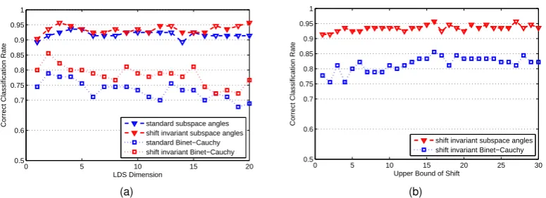
0 5 10 15 20 0.5
0.6 0.7 0.75 0.8 0.85 0.9 0.95 1
LDS Dimension
Correct Classification Rate standard subspace angles shift invariant subspace angles standard Binet−Cauchy shift invariant Binet−Cauchy
(a)
0 5 10 15 20 25 30
0.5 0.6 0.7 0.75 0.8 0.85 0.9 0.95 1
Upper Bound of Shift
Correct Classification Rate
shift invariant subspace angles shift invariant Binet−Cauchy
(b)
Fig. 9. Evaluation of robust LDS dimension n (a), and upper bound of temporal shift T (b). The
performance of shift invariant and standard distance metrics is illustrated for comparison.
behaviors, which are categorized into 13 different actions. Each scene is recorded both from top-view
and side-view using two fixed, synchronized cameras. Each video lasts about 10 minutes, for a total
of over 88 hours of video and 8 million frames. We follow the original experimental setup by using
104 videos for training and 133 for test. We report average accuracy over all classes as performance.
6.3 Experiments on Short Clips Datasets
6.3.1 Evaluation of Robust LDS Dimension
In Fig. 9a, we examine the relationship between the correct classification rate (CCR) and the model
dimension n up to 20 using only global dynamics on the Weizmann dataset. We also evaluate the
performance of our proposed shift invariant distance metric compared with the standard subspace
angles distance and the Binet-Cauchy kernel. The kernel distance is computed as
d(M1,M2) =k(M1,M1) +k(M2,M2)−2k(M1,M2)
We see that: 1) the recognition rate does not improve much with the increase of model dimensionn
for the shift invariant and standard subspace angles distance (see Fig. 9a ’triangle’ data). This means
that we can choose a comparatively small model dimension, sayn= 3, to gain a large saving of
com-putation expense with only a small reduction in the recognition rate; 2) the recognition rate even drops
with the increase of model dimensionnfor the shift invariant and standard Binet-Cauchy kernel (see
Fig. 9a ’square’ data). This indicates that the Binet-Cauchy kernel is not suitable for high-dimensional
linear dynamical models; 3) the proposed shift invariant distance/kernel always performs better than
the standard subspace angles distance and the Binet-Cauchy kernel (see Fig. 9a, red vs. blue). The
shift invariant/standard subspace angles distance performs better than the shift invariant/standard
Binet-Cauchy kernel (see Fig. 9a, triangle vs. square); 4) the proposed shift invariant subspace angles
distance outperforms the other three distance metrics and achieves a best recognition result of 95.70%
with n= 3. So in the following experiments, we use the shift invariant subspace angles distance as
default metric for LDS unless otherwise specified.
6.3.2 Evaluation of Upper Bound of Shift
In Fig. 9b, we evaluate the recognition performance with respect to upper bound of temporal shift
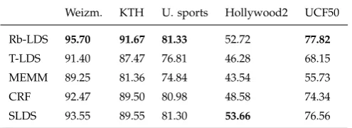
[image:20.595.105.493.68.209.2]TABLE 1
Comparison of different temporal models (%)
Weizm. KTH U. sports Hollywood2 UCF50
Rb-LDS 95.70 91.67 81.33 52.72 77.82
T-LDS 91.40 87.47 76.81 46.28 68.15
MEMM 89.25 81.36 74.84 43.54 55.73
CRF 92.47 89.50 80.98 48.58 74.34
SLDS 93.55 89.55 81.30 53.66 76.56
increasing of temporal shift does not yield better results. In addition, with the increase in T, the
computational cost increases dramatically. Considering that most of the concerned sequences are
non-periodic or have only short periods, we chooseT = 16in all the experiments.
6.3.3 Comparison of Different Temporal Models
The different temporal models are compared in Table 1. We see that robust LDS (Rb-LDS) consistently
outperforms the other models on all the datasets except switching LDS (SLDS) on the Hollywood2
dataset.
Rb-LDS gives an average 3%-9% improvement over the traditional LDS (T-LDS). This indicates
that the stability criterion of dynamical systems plays an important role in the results. For T-LDS, the
computation of the shift invariant distance metric may fail if the LDS is degenerate. This is especially
clear on the realistic datasets, e.g., UCF sports, Hollywood2 and UCF50, because they contain many
more disturbance factors.
Notwithstanding all these disadvantages, T-LDS outperforms MEMM by nearly 2%-12% because
it captures the global dynamics. CRF gives much better results than both T-LDS and MEMM. This
is probably because CRF considers the temporal context. It is interesting to notice that the temporal
context is especially useful to discriminate actions with a similar motion style, e.g., walk vs. jog in
the KTH dataset. However, training CRF with a long window of observations is much more time
consuming than for T-LDS and MEMM.
SLDS achieves a recognition performance almost as good as Rb-LDS. These two methods both use
LDS to describe the sequence dynamics. SLDS further builds a stochastic model on top of a set of
LDSs. The switching or transition among the set of LDSs describes the nonlinear dynamics. This is
why SLDS gives a slightly better result on the more complex dataset, e.g., Hollywood2, in which many
clips include multiple primitive actions. However, Rb-LDS consistently performs better than SLDS on
the other datasets, because Rb-LDS specifically considers the stability of the LDS and temporal shifts
of the action sequence. In addition, learning SLDS involves many more parameters and exact inference
is generally not possible. On the other hand, training Rb-LDS is simple and efficient. Classification is
achieved by directly defining a distance metric on the LDS space. This makes it straightforward to
compare two action sequences. More importantly, Rb-LDS yields a pairwise distance matrix, which
can be embedded into the maximum margin distance learning framework. This embedding cannot
A closely related LDS-based activity clustering method is proposed by Turaga et al. [20], who
consider the same tools as ours and SLDS. They segment a long video sequence into meaningful
subsequences by searching for action boundaries with a suboptimal algorithm. Then they fit LDSs
to each segment and cluster them by building a distance metric on LDSs. Each clustering center
represents an action component, and each LDS is assigned the label to its nearest center. The sequence
is finally modeled as a cascade of LDSs (CLDS). CLDS differs with SLDS in two ways. First, CLDS
assumes as given the number of clustering centers to model action components, while SLDS assumes
the number of hidden states. Second, CLDS maintains the temporal structure of LDSs using an
n-grams model, while SLDS maintains the temporal structure with a state transition matrix. The
similarity between Rb-LDS and CLDS is that they both use LDS to describe motion dynamics and
define a distance metric on LDSs. However, CLDS differs with Rb-LDS in that it is designed to
mine repetitive patterns from long sequences which may contain multiple activities. To define and
search for a stable segmentation boundary in long sequences is indeed not so straightforward. The
success of the search largely depends on the definition of action components and the expected
segmentation granularity. The proposed reconstruction error based algorithm [20] indeed produces
many uncertainties in the segmentation. These uncertainties can be eliminated or alleviated by our
proposed aligned distance metric.
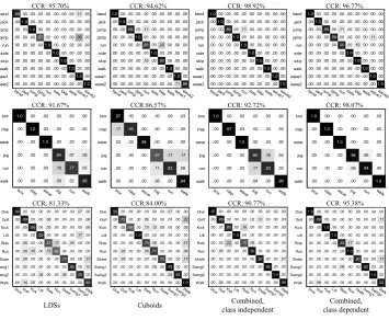
6.3.4 Recognition Performance of Proposed Framework
In Fig. 10, we compare confusion matrices with respect to different distance measures: LDSs, cuboids
and combined distances with both class independent and class dependent weights on three action
datasets, namely Weizmann, KTH and UCF sports. For Hollywood2, binary classification is carried
out for each action class as all the clips are labeled with 1 or -1, indicating whether the clip contains
a specific action class or not. For this reason, we only conduct class independent combination for
each action class separately and show the results in Table 2, accompanied with the learned class
independent weights for each class. The class dependent combination is not applicable for this dataset.
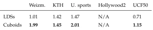
For UCF50, since it contains 50 action classes, we only show the average results in Table 3 due to
limited space. We also give the class independent weights in Table 4 and class dependent weights in
Fig. 11 on all the datasets.
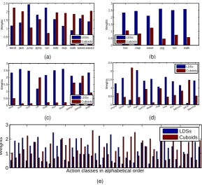
We see that LDSs give fairly good results by themselves, and outperform cuboids on all the datasets
except the UCF sports. It is worth noting that the recognition rates achieved by LDSs are nearly 10%
better than those obtained by cuboids on Hollywood2 and UCF50. This indicates that LDSs are
more discriminative than cuboids on complex datasets which contain large temporal variations. The
UCF sports dataset involves many specific environments and items of equipment. Local cuboids are
designed to capture this information, and thus achieve better results on this dataset.
We observe that the combination of LDSs and cuboids significantly improves the final performance
for both class independent and class dependent modes on all the datasets. In general, the class
dependent combinations achieve better results than the class independent combinations. This is