Splitting of Traffic Flows to Control Congestion in Special Events

(1)

Volume 2011, Article ID 563171,18pages doi:10.1155/2011/563171

Research Article

Splitting of Traffic Flows to Control Congestion in

Special Events

Ciro D’Apice, Rosanna Manzo, and Luigi Rarit `a

Dipartimento di Ingegneria Elettronica e Ingegneria Informatica, Universit`a degli Studi di Salerno, Via Ponte Don Melillo, 84084 Fisciano, Italy

Correspondence should be addressed to Rosanna Manzo,[email protected]

Received 24 December 2010; Accepted 12 February 2011

Academic Editor: Marianna Shubov

Copyrightq2011 Ciro D’Apice et al. This is an open access article distributed under the Creative Commons Attribution License, which permits unrestricted use, distribution, and reproduction in any medium, provided the original work is properly cited.

We deal with the optimization of traffic flows distribution at road junctions with an incoming road and two outgoing ones, in order to manage special events which determine congestion phenomena. Using a fluid-dynamic model for the description of the car densities evolution, the attention is focused on a decentralized approach. Two cost functionals, measuring the kinetic energy and the average travelling times, weighted with the number of cars moving on roads, are considered. The first one is maximized with respect to the distribution coefficient, and the second is minimized with respect to the same control parameter. The obtained results have been tested by simulations of urban networks. Decongestion effects are also confirmed estimating the time a car needs to cross a fixed route on the network.

1. Introduction

(2)

A

B

[image:2.600.171.431.102.210.2]

C

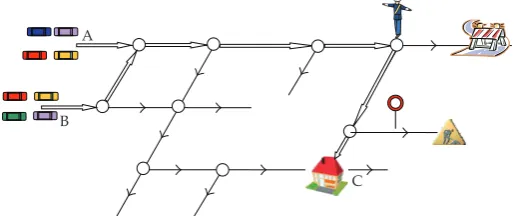
Figure 1: Example of car flows redistribution.

In this context, using a fluid dynamic model able to foresee the traﬃc density evolution on road networks see 1–4, we propose a strategy to redistribute in an optimal way flows at junctions. According to the adopted model, the car densities on each road follow a conservation law see 5, while dynamics at junctions is uniquely solved using the following rules:

Athe incoming traﬃc at a node is distributed to outgoing roads according to some distribution coeﬃcients;

Bdrivers behave so as to maximize the flux through the junction.

If a junctionJis of 1×2 typenamely, one incoming road, 1, and two outgoing ones, 2 and 3, ruleAis expressed by a distribution parameterα, indicating the percentage of cars going from road 1 to road 2. Assigning initial densities for incoming and outgoing roads and using ruleB, we finally compute the asymptotic solution as function ofα.

Here, considering the distribution coefficient as control parameter, we aim to redirect traffic at junctions of 1×2 type in order to improve urban traffic and face emergency situations. In particular, we analyze two optimization problems over a fixed time horizon: minimizing an objective functionW1, estimating the kinetic energy; maximizing a functionalW2, measuring the average travelling time of drivers, weighted with the number of cars moving on roads. Indeed, we prove that both functionals are optimized for the same value ofα.

Some control strategies for the right of way parameters and distribution coeﬃcients have already been treated in6,7, where three cost functionals, related to average velocity, average travelling time, and flux, have been introduced for 1×2 and 2×1 junctions. Cost functionalsW1 andW2 have been studied in8 for the optimal control of green and red phases of traﬃc lights, while in9parameters of 2×2 junctions have been optimized for the fast transit of emergency vehicles along an assigned path in case of car accidents.

The analysis of the functionalsW1 and W2on a whole network is a very hard task, so we follow a decentralized approach: an exact solution is found for single 1×2 junctions and asymptoticW1 andW2. The global suboptimal solution for networks is obtained by localization: the exact optimal solution is applied locally for each time at each junction of 1×2 type.

The analytical optimization results are then tested by simulationsfor numerics, see

(3)

Simulation results for a symmetric topology show that, assuming random distribution coefficients, the congestion of one road can determine high traffic densities on the whole network, while decongestion phenomena occur when optimalαvalues are used. In the case study of a portion of the Salerno urban network in Italy, characterized by an asymmetric topology, with 1×2 and 2×1 junctions, some interesting aspects arise: random coefficients frequently provoke hard congestions, as expected; optimal distribution coefficients allow a local redistribution of traffic flows. While random simulation curves of the cost functionalW1 are always lower than the optimal one, the optimal curve ofW2is higher than some random ones. This is not surprising because, at 2×1 junctions, traffic densities can remain high. Hence, for such a network,locallyoptimal solutions alleviate critical traffic situations, but the aim of the global optimization ofW1andW2is not achieved. Moreover, using an algorithmsee

13for tracing car trajectories on a network, some simulations are run to test how the total travelling time of a driver is influenced by distribution coeﬃcients. As intuition suggests, the time for covering a path of a single driver decreases when optimalαvalues are used.

The paper is organized as follows. Section2is devoted to the description of the model for road networks and to the construction of solutions to Riemann Problems 1×2 junctions. In Section3, we define the cost functionalsW1 and W2 and optimize them with respect to the distribution coeﬃcients at a single junction. Simulation results for complex networks are presented in Section4. Section5ends the paper through conclusions.

2. A Riemann Solver for Road Networks

A road network is described by a coupleI,J, whereIrepresents the set of roads, modelled by intervalsai, bi⊂Ê,i1, . . . , N, andJis the collection of junctions.

Indicating byρ ρt, x ∈ 0, ρmax the density of cars,ρmax the maximal density, fρ ρvρthe flux withvρthe average velocity, the traﬃc dynamics is described on each road by the conservation lawLighthill-Whitham-Richards model,3,4:

∂tρ ∂xf

ρ0. 2.1

We assume that:Ffis a strictly concaveC2_{function such that}_f₀ _f_ρ

max 0. Choosingρmax1 andvρ 1−ρ, a flux function ensuringFis

fρρ1−ρ, ρ∈0,1, 2.2

which has a unique maximumσ1/2.

In order to capture the dynamics at a junction, we solve Riemann Problems RPs, Cauchy Problems with a constant initial datum for each incoming and outgoing road, the basic ingredient for the solution of Cauchy Problems by Wave-Front-Tracking algorithms.

Consider a junctionJ ofn×mtype, that is, withnincoming roadsIϕ,ϕ1, . . . , n, m outgoing roads,Iψ,ψ n 1, . . . , n m, and initial datumρ0 ρ1,0, . . . , ρn,0, ρn 1,0, . . . , ρn m,0.

Definition 2.1. A Riemann Solver RSfor the junction J is a map RS : 0,1n×0,1m →

(4)

We require the following conditions hold true: C1 RSRSρ0 RSρ0; C2 on each incoming roadIϕ,ϕ1, . . . , n, the waveρϕ,0,ρϕhas negative speed, while on each outgoing roadIψ,ψn 1, . . . , n m, has the waveρψ, ρψ,0has positive speed.

Ifm≥n, a possible RS atJis defined by the following rulessee1:

Atraffic is distributed at J according to some coefficients, collected in a traffic distribution matrix A αj,i, i 1, . . . , n, j n 1, . . . , n m, 0 < αj,i < 1,

_n _m

jn 1αj,i 1. Theith column ofAindicates the percentages of traﬃc that, from the incoming roadIi, distribute to the outgoing roads;

BfulfillingA, drivers maximize the flux throughJ.

Focus on a 1×2 junctionJ. We indicate the cars density on the incoming road 1 by ρ1t, x ∈ 0,1,t, x ∈Ê ×I1, and on the outgoing roadsψ,ψ 2,3, by ρψt, x ∈ 0,1,

t, x∈Ê ×Iψ.

Consider the flux function2.2and letρ1,0, ρ2,0, ρ3,0be the initial densities atJ. The maximal flux values on roads are defined by

γmax 1 ⎧ ⎪ ⎪ ⎨ ⎪ ⎪ ⎩

fρ1,0

if 0≤ρ1,0≤ 1 2, f 1 2 if 1

2 ≤ρ1,0≤1,

γmax ψ ⎧ ⎪ ⎪ ⎨ ⎪ ⎪ ⎩ f 1 2

if 0≤ρψ,0≤ 1

2, ψ 2,3, fρψ,0

if 1

2 ≤ρψ,0≤1, ψ 2,3.

2.3

Ifα∈0,1and 1−αindicate, respectively, the percentage of cars that, from road 1, goes to the outgoing roads 2 and 3, the fluxes solution to the RP atJare

γγ1, αγ1,1−αγ1

, 2.4

where

γ1min

γ₁max,γ max 2

α , γmax

3 1−α

. 2.5

Hence,ρf−1_γ_{is found as follows}_see₁_,₂_:

ρ1∈

⎧ ⎪ ⎪ ⎨ ⎪ ⎪ ⎩

ρ1,0

∪τρ1,0

,1 if 0≤ρ1,0≤ 1 2,

1 2,1

if 1

2 ≤ρ1,0≤1,

ρψ∈

⎧ ⎪ ⎪ ⎨ ⎪ ⎪ ⎩ 0,1 2

if 0≤ρψ,0≤ 1

2, ψ2,3,

ρψ,0

∪0, τρψ,0

if 1

2 ≤ρψ,0≤1, ψ2,3,

(5)

whereτ :0,1 → 0,1is the map such thatfτρ fρfor everyρ∈0,1andτρ/ρ for everyρ∈0,1\ {1/2}.

Finally, on the incoming road 1, the solution is given by the waveρ1,0,ρ1, while on the outgoing roadψ,ψ2,3, the solution is represented by the waveρψ , ρψ,0.

3. Distribution Parameters Optimization

Fix a 1×2 junctionJand an initial datumρ1,0, ρ2,0, ρ3,0. We define the cost functionalW1t andW2t, which measure, respectively, the kinetic energy and the average travelling time weighted with the number of cars moving on roads:

W1t 3

k1

Ik

fρkt, x

vρkt, x

dx,

W2t 3

k1

Ik

ρkt, x vρkt, x

dx.

3.1

For a fixed time horizon 0, T, with T sufficiently big, consider the traffic distribution coefficientαas control. We aim to maximizeW1Tand to minimizeW2Tseparately. The functionals assume the form:

W1T 3

i1 fρi

vρi

1

2 3

i1

γi

1−si

1−4γi

,

W2T 3

i1

ρi vρi

3

i1 1 si

1−4γi

1−si

1−4γi ,

3.2

wheres1andsψ,ψ 2,3, are given by

s1 ⎧ ⎪ ⎪ ⎪ ⎪ ⎪ ⎪ ⎪ ⎪ ⎪ ⎪ ⎨ ⎪ ⎪ ⎪ ⎪ ⎪ ⎪ ⎪ ⎪ ⎪ ⎪ ⎩

1 ifρ1,0≥ 1 2,

orρ1,0< 1 2 and γ

max 1 >min

_γmax 2

α , γmax

3 1−α

,

−1 ifρ1,0< 1 2 andγ

max

1 ≤min

_γmax 2

α , γmax

3 1−α

, sψ ⎧ ⎪ ⎪ ⎪ ⎪ ⎪ ⎪ ⎪ ⎪ ⎪ ⎪ ⎨ ⎪ ⎪ ⎪ ⎪ ⎪ ⎪ ⎪ ⎪ ⎪ ⎪ ⎩

1 ifρψ,0> 1 2 and

γ_ψmax αψ ≤

min

γmax 1 ,

γ_ψmax

αψ

, ψ/ψ,

−1 ifρψ,0≤ 1 2,

orρψ,0> 1 2 and γmax ψ αψ >min γmax 1 , γmax ψ αψ

, ψ/ψ,

(6)

with

αψ

⎧ ⎨ ⎩

α ifψ 2,

1−α ifψ 3. 3.4

According to the solution of the RP atJ, we have

W1T

γ1 2

1−s1

1−4γ1

_α_γ

1 2

1−s2

1−4αγ1

₁₋_α_γ

1 2

1−s3

1−41−αγ1

,

W2T

1 s1

1−4γ1

1−s1

1−4γ1

1 s2

1−4αγ1

1−s2

1−4αγ1

1 s3

1−41−αγ1

1−s3

1−41−αγ1 ,

3.5

whereγ1is given by2.5. The values ofα, which optimizeW1TandW2T, are reported in the following theoremfor the sketch of the proof, see the appendix.

Theorem 3.1. Fix a 1×2 junctionJ. AssumingTsuﬃciently big, the cost functionalsW1TW2T

is maximized (minimized) forα1/2, with the exception of the following cases (for some of them, the

optimal control does not exist but it is approximated):

aifγmax

3 ≤γ1max/2< γ1max≤γ2max,αα1 ε;

bifγ₂max< γ₁max/2< γ₁max≤γ₃max,αα2;

cifγ₂max< γ₃max< γ₁max, we distinguish three subcases:

c1ifγ₁max−γ₃max≥γ₂max,αα3;

c2ifγ₁max−γ₃max< γ₂maxγ₁max/2,α 1/2−ε;

c3ifγmax

1 −γ3max< γ2max≤γ1max/2,αα2−ε;

difγmax

3 < γ2max< γ1max, we distinguish two subcases:

d1ifγ₁max−γ₃max≥γ₂max,αα3 ε;

d2if1/2γmax

1 ≤γ1max−γ3max< γ2max,αα1−ε,

whereα1 γ₁max−γ₃max/γ₁max,α2 γ₂max/γ₁max,α3 γ₂max/γ₂max γ₃maxand εis small and

positive.

Example 1. Discuss the optimal solution for the following initial conditions:

Aρ1,00.35,ρ2,00.2,ρ3,00.9;

Bρ1,00.45,ρ2,00.75,ρ3,00.15;

Cρ1,00.3,ρ2,00.9,ρ3,00.8.

In caseA, we get

(7)

W1T

α1 1

α

a

W2T

α1 1

α

[image:7.600.139.459.96.215.2]

b

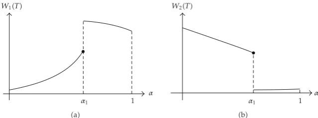
Figure 2: CaseA: behaviour ofW1andW2for suﬃciently big.

so conditionγ₃max< γ₁max< γ₂maxis satisfied. Hence,

, 3.7

where

γ1

⎧ ⎪ ⎪ ⎨ ⎪ ⎪ ⎩

γmax 3

1−α, 0< α≤α1,

γ₁max, α1< α <1,

3.8

withα1 0.6. ForTsuﬃciently big,W1TandW2Thave one discontinuity point atαα1, as shown in Figure2. The optimal control does not exist, but one can chooseαα1 ε.

In caseB, we have that

γ₁max0.2475, γ₂max0.1875, γ₃max0.25, 3.9

hence conditionγmax

2 < γ1max< γ3maxholds. Then, the solution to the RP atJis

, 3.10

where

γ1

⎧ ⎪ ⎪ ⎪ ⎨ ⎪ ⎪ ⎪ ⎩

γmax

1 , 0< α≤α2,

γmax 2

α , α2< α <1,

3.11

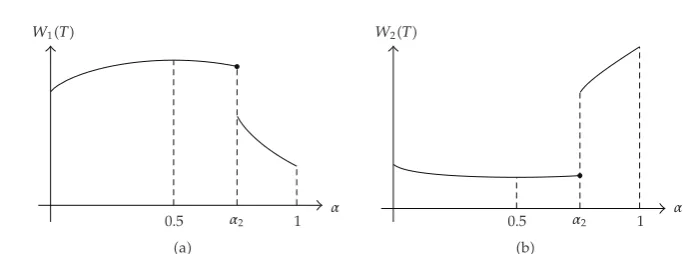
with α2 0.7575. For T suﬃciently big, the cost functionals W1T and W2T have one discontinuity point at α α2, as shown in Figure 3. The optimal control exists, and it is α1/2, for which

(8)

W1T

0.5 α2 1

α

a

W2T

0.5 α2 1

α

[image:8.600.121.463.86.213.2]

b

Figure 3: CaseB: behaviour ofW1andW2forTsuﬃciently big.

W1T

α1 α2 1

α

a

W2T

α1 α2 1

α

[image:8.600.141.463.253.371.2]

b

Figure 4: CaseC: behaviour ofW1andW2forT suﬃciently big.

In caseC

γ₁max0.21, γ₂max0.09, γ₃max0.16, 3.13

hence conditionγ₂max< γ₃max< γ₁maxis satisfied, and we obtain

, 3.14

where

γ1

⎧ ⎪ ⎪ ⎪ ⎪ ⎪ ⎪ ⎪ ⎪ ⎪ ⎨ ⎪ ⎪ ⎪ ⎪ ⎪ ⎪ ⎪ ⎪ ⎪ ⎩

γ₃max

1−α, 0< α≤α1,

γ₁max, α1< α < α2,

γmax 2

α , α2< α <1,

3.15

(9)

a

1

b

c

2

3

[image:9.600.229.373.100.183.2]

g f e d

Figure 5: Topology of the symmetric network.

4. Road Traffic Simulation

We present some simulation results in order to test the optimization algorithm for the cost functionals. In particular, we analyze the eﬀects of diﬀerent control procedures, applied locally at each junction, on the global performances of networks and compute the travelling time of a car on assigned paths. For simplicity, from now on we drop the dependence onT fromW1andW2.

4.1. A Symmetric Network

In this subsection, we analyze a symmetric network with three simple junctions of 1×2 type, labelled by 1, 2, and 3, see Figure 5. In particular, the network consists of two inner roads,bandc, and five roads, that connect the inner roads to outside:a,d,e,f, andg. The conservation law with flux function2.2is approximated using the Godunov scheme, with space stepΔx0.0125, and time step, determined by the CFL conditionsee10,11, equal to 0.5. We assume initial conditions zero for all roads at the starting instant of simulation

t0, a 0.3 Dirichlet boundary datum for roadsa,d,e,f, a 0.9 Dirichlet boundary condition for roadgand a time interval of simulation0, T, whereT 30 min.

Two diﬀerent choices of the distribution coeﬃcients are considered:locallyoptimal parameters at each junction, given by analytical resultsoptimal case; random parameters

random case, that is, the distribution coeﬃcients are taken randomly for each road junction

when the simulation starts and then are kept constant.

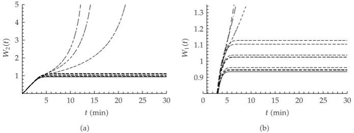
The evolution of W1 and of W2 are depicted in Figures 6 and 7, reporting with a continuous line the optimal case and with dashed lines various random cases. In some random simulations, the α values are such that a lower traﬃc density goes to road g, with a consequent natural improvement of the network performances. This justifies the fact that some dashed W1 and W2 curves approach the optimal ones. In other cases, W1 rapidly decreases andW2tends to infinity, indicating that the random choice ofαprovokes congestions on all network roads. However, in any case, the optimal case is better than the others. In fact, it describes the natural situationthat happens on congested real urban networksin which the traﬃc is redirected to less congested roads.

4.2. A Real Urban Network

(10)

0.1 0.2 0.3 0.4 0.5

W1

t

5 10 15 20 25 30

tmin

a

0.42 0.44 0.46 0.5 0.48 0.52 0.54

W

1

t

5 10 15 20 25 30

tmin

[image:10.600.117.482.88.229.2]

b

Figure 6: W1t evaluated for optimal distribution coeﬃcients continuous line and random choices

dashed lines.aevolution in0;T.bzoom around the asymptotic optimal values.

1 2 3 4 5

W

2

t

5 10 15 20 25 30

tmin

a

0.9 1 1.1 1.2 1.3

W

1

t

0 5 10 15 20 25 30

tmin

b

Figure 7: W2t evaluated for optimal distribution coeﬃcients continuous line and random choices

dashed lines.aevolution in0;T.bzoom around the asymptotic optimal values.

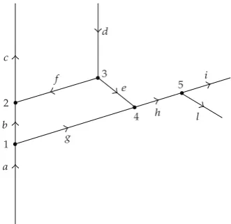
Via Leonino Vinciprovasegmentsdande, Via Settimio Mobiliosegmentsf,g,h, andi, and Via Guerciosegment l. We distinguish inner roads segments, b,e,f,g, andh, and external ones,a,c,d,i,l. Junctionsindicated by numbers1, 3 and 5 are of 1×2 type,while 2 and 4 are of 2×1 types. The evolution of traﬃc flows is simulated by the Godunov method withΔx 0.0125,Δt Δx/2 in a time interval0, T, withT 120 min. Initial conditions and boundary data for densities are in Table1and have been taken in order to simulate a congestion scenario. Notice that, for junctions 2 and 4, right of way parameters are chosen according to measures on the real network.

[image:10.600.126.474.276.407.2]

(11)

a

1

b

2

c

f

g

4 h 5 i

l

3

d

[image:11.600.216.382.97.258.2]

e

Figure 8: Topology of the portion of the real urban network of Salerno.

0.2 0.4 0.6 0.8 1

W

1

t

20 40 60 80 100 120

tmin

a

20 40 60 80 100 120 140

W

2

t

20 40 60 80 100 120

tmin

[image:11.600.123.478.303.436.2]

b

Figure 9: Evolution in0;T ofW1t a andW2t b evaluated for optimal distribution coeﬃcients

continuous lineand random choicesdashed lines.

Table 1: Initial conditions, boundary data and right of way parameters for roads of the network.

Road Initial condition Boundary data Right of way parameters

a 0.2 0.3 /

b 0.2 / 0.2

c 0.2 0.9 0.4

d 0.2 0.3 /

e 0.8 / /

f 0.2 / 0.8

g 0.75 / 0.6

h 0.6 / /

i 0.75 0.9 /

l 0.75 0.9 /

[image:11.600.100.504.506.642.2]

(12)

0.2 0.4 0.6 0.8 1

x

t

22.5 25 27.5 30 32.5 35 37.5

tmin

a

0.2 0.4 0.6 0.8 1

x

t

62.5 65 67.5 70 72.5 75 77.5

tmin

[image:12.600.115.480.73.230.2]

b

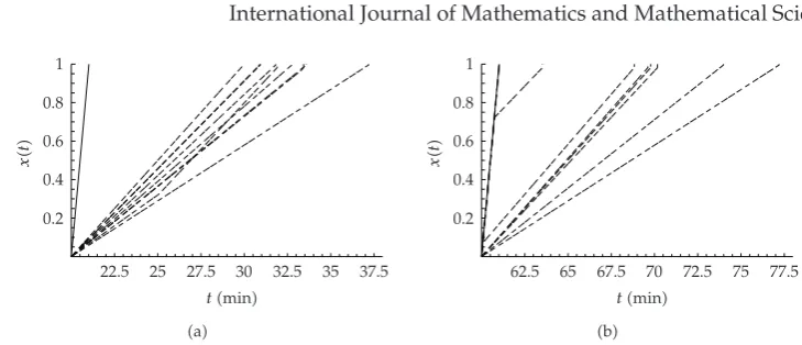
Figure 10: Evolution of a car trajectoryxtalong roadgwith initial travel timest0 20aandt0 60

b, evaluated for optimal distribution coeﬃcientscontinuous linesand random choicesdashed lines.

distribution coefficients are used, high traffic densities affect some roads and this justifies that the optimal curve is not the lowest forW2.

Suppose that a car travels along a path in a network, whose traﬃc evolution is modeled by2.1. The position of the driverxxtis obtained solving the Cauchy problem:

˙

xvρt, x,

xt0 x0,

4.1

wherex0is the initial position at the initial timet0, whilev1−ρ. Using numerical methods, described in13, we aim to estimate the driver travelling time and to prove the goodness of the optimization results. First, we compute the car trajectory along roadg and the time needed for covering it in optimal case and random cases; then, we fix a car path within the Salerno network and study the exit time evolution versus the initial travel timet0the time in which the car enters into the network.

In Figure 10, we assume that the car starts its own travel at the beginning of road g at the initial times t0 20a and t0 60band compute the trajectories xt along roadg, in optimal casecontinuous lineand random casesdashed lines. Although initial timest0are diﬀerent, the evolutionxtin the optimal case has always a higher slope with respect to trajectories in random cases because traﬃc levels are low. When random choices of parametersαare used, higher boundary conditions for roadsc,i, andlcause an increase in density values by shocks propagating backwards. Hence, car velocities are reduced, travel times become longer and so exit times from roadg.

In Table2, we collect the exit timesTout from roadgthe times needed to go out from roadg, for the optimal choice of distribution coeﬃcientsoptand random choicesri,i 1, . . . ,9, assumingt020.

(13)

[image:13.600.187.413.114.258.2]

Table 2: Initial conditions, boundary data and right of way parameters for roads of the network.

Simulations Tout

opt 1.02

r1 9.955

r2 10.89

r3 10.93

r4 11.82

r5 11.895

r6 12.75

r7 13.43

r8 13.585

r9 17.185

2 4 6 8 10 12 14

Texit

t

10 20 30 40 50 60 70 80

t0min

a

10 20 30 40

Texit

t

10 20 30 40 50 60 70 80

t0min

b

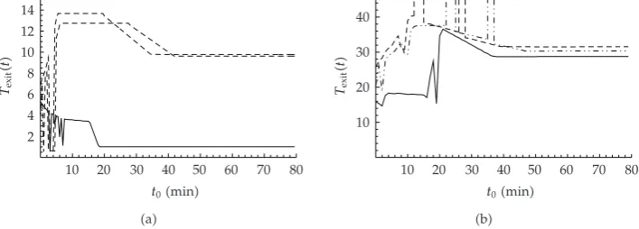
Figure 11: Exit time from road g versus initial travel time t0in 0,80 a and exit time from the

patha, g, h, lversus initial travel timest0 in0,80 b, evaluated for optimal distribution coeﬃcients

continuous linesand random choicesdashed and dot dashed lines.

Finally, in Figure11b, we consider the exit timeTouttfrom a fixed route,a, g, h, l, versus the initial times t0. Precisely, we study the temporal variation of Tout when a car, starting its trip at the beginning of roadaat timet0, crosses roadsa,g,h,lin order to exit from the network. Also in this case, different choices of distribution coefficientsthe optimal one is indicated by a continuous line, unlike the othersaffect the time for covering the path. When optimal parameters are not used,Touttends to infinity at some critical timestctc 13 andtc 27 for the random case represented by dashed line, andtc 23 andtc 36 for the random case with dot-dashed line. This occurs because the car cannot enter roadgor road h, since the traffic within them is blocked. For times greater than critical ones, traffic densities become stablea light decongestion allows the car to reach the destinationand exit times reach a steady valueTout 31.5 andTout 30.35at times, respectively,t0 42 andt0 46. On the contrary, when optimal parameters are used, the exit time does not tend to infinity

as the network is never congestedand reaches the steady valueTout 28.75 at timet0 38

[image:13.600.123.477.302.429.2]

(14)

γ1

α1 1 α

γmax

1

γmax

3 1−α

γmax

2

α

a

γ1

α2 1 α

γmax

1

γmax

3 1−α

γmax

2

α

[image:14.600.133.458.91.212.2]

b

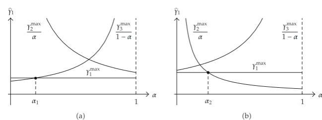
Figure 12:acaseγ₃max< γ₁max< γ₂max.bcaseγ₂max< γ₁max< γ₃max.

5. Conclusions

In this paper, an optimization study has been presented to improve the urban traﬃc condi-tions in case of special events in which splitting of flows is needed.

The optimization has been made over traffic distribution coefficients at junctions, using two cost functionals, that measure, respectively, the kinetic energy and the average travelling times of drivers, weighted with the number of cars moving on roads. An exact solution has been found for simple junctions having one incoming road and two outgoing roads. The obtained analytical results have been tested through simulations, showing that in some cases a total decongestion effect is possible. This is also confirmed by evaluations of cars trajectories on some roads and fixed routes on the network: using optimal distribution coefficients, times needed to cover paths are the lowest.

Appendix

We report the proof of Theorem3.1. Consider new functionals, W1 and W2, in which the terms not depending on αare neglected. Since the solution to the RP atJ depends on the value of the parameterα, we distinguish various cases. Here, for sake of brevity, we analyze some of them.

Assumesee Figure12athat

γ₃max< γ₁max< γ₂max, A.1

then

γ1

⎧ ⎪ ⎪ ⎪ ⎨ ⎪ ⎪ ⎪ ⎩

γmax 3

1−α, 0< α≤α1,

γ₁max, α1< α <1,

(15)

whereα1 γ₁max−γ₃max/γ₁max. As for 0 < α ≤ α1,s1 1, s2 −1, and forα1 < α < 1, s2s3−1,W1andW2assume the form:

W1 ⎧ ⎪ ⎪ ⎪ ⎪ ⎪ ⎨ ⎪ ⎪ ⎪ ⎪ ⎪ ⎩ 1 1−α

⎛ ⎝₁₋

1−4γ max 3 1−α

⎞ ⎠ α

1−α

1

1−4 α 1−αγ

max 3

, 0< α≤α1,

α1 1−4αγmax

1 1−α

1 1−41−αγmax

1 , α1 < α <1,

W2 ⎧ ⎪ ⎪ ⎪ ⎪ ⎪ ⎪ ⎪ ⎪ ⎪ ⎨ ⎪ ⎪ ⎪ ⎪ ⎪ ⎪ ⎪ ⎪ ⎪ ⎩

1 1−4γmax

3 /1−α

1−1−4γmax

3 /1−α

1−1−4α/1−αγ₃max

1 1−4α/1−αγ₃max

, 0< α≤α1,

1−

1−4αγ₁max

1 1−4αγmax 1

1−

1−41−αγ₁max

1

1−41−αγ₁max

, α1< α <1.

A.3

Our aim is to maximizeW1and to minimizeW2separately with respect to the parameterα. If 0< α≤α1, then

∂W1 ∂α 2

γmax 3

1−α3

1 μ1−α−

α μ1−α/α

1

1−α2

2−μ1−α μ

1−α α , ∂W2 ∂α 4γmax 3

μ1−α/α1 μ1−α/α21−α2 −

4γmax 3

μ1−αμ1−α−121−α2,

A.4

whereμα 1−4γmax

3 /1−α, and hence the functionalsW1andW2are, respectively, an increasing and a decreasing function.

Ifα1< α <1, we get

∂W1 ∂α 2γ

max 1

η1−α−ηα ζα−ζ1−α,

∂W2 ∂α 2γ

max 1

χα−χ1−α θα−θ1−α,

A.5

where

ζα

1−4αγ₁max, ηα α ζα,

χα 1−ζα

1 ζα2ζα, θα

1

1 ζαζα.

(16)

Since

∂W1

∂α ≥0⇐⇒α∈

0,1 2

, ∂W2

∂α ≥0⇐⇒α∈

1 2,1

, A.7

we conclude thatW1andW2are maximized and minimized, respectively, forα1/2. Finally, we obtain that

iifα1<1/2, for allα∈0, α1∪α1,1/2,

∂W1 ∂α ≥0,

∂W2

∂α ≤0; A.8

iiifα1≥1/2, for allα∈0, α1,

∂W1 ∂α >0,

∂W2

∂α <0. A.9

Moreover,

lim α→α₁

!

W1α−W1α1

"

>0, lim α→α₁

!

W2α1−W2α

"

>0. A.10

Hence, we conclude that

iifα1<1/2,W1andW2are optimized forα1/2;

iiifα1 ≥ 1/2, the optimal value for bothW1andW2does not exist. One can choose αα1 ε, withεsmall and positive constant.

In the particular caseγ₃max < γ₁max γ₂max, the analysis is unchanged. Ifγ₁max γ₃max < γ₂maxbothW1andW2are optimized forα1/2.

Assume thatFigure12b

γmax

2 < γ1max< γ3max. A.11

We have

γ1

⎧ ⎪ ⎪ ⎪ ⎨ ⎪ ⎪ ⎪ ⎩

γ₁max, 0< α≤α2,

γ₂max

α , α2< α <1,

(17)

whereα2 γ₂max/γ₁max. Then, as for 0 < α ≤ α2,s2 s3 −1, and for α2 < α < 1,s1 1, s3−1, we have to maximize

W1 ⎧ ⎪ ⎪ ⎪ ⎪ ⎪ ⎪ ⎪ ⎨ ⎪ ⎪ ⎪ ⎪ ⎪ ⎪ ⎪ ⎩ α

1−4αγ₁max 1−α

1−41−αγ₁max, 0< α≤α2,

1 α

⎛ ⎝₁₋

1−4γ max 2

α

⎞ ⎠ 1−α

α

#

1

1−41−α α γ

max 2

$

, α2< α <1,

A.13

and to minimize

W2 ⎧ ⎪ ⎪ ⎪ ⎪ ⎪ ⎪ ⎪ ⎪ ⎪ ⎪ ⎨ ⎪ ⎪ ⎪ ⎪ ⎪ ⎪ ⎪ ⎪ ⎪ ⎪ ⎩

1−1−4αγmax 1

1 1−4αγmax 1

1−1−41−αγmax 1

1 1−41−αγmax 1

, 0< α≤α2,

1

1−4γ₂max/α

1−

1−4γ₂max/α

1−1−41−α/αγmax 2

1 1−41−α/αγ₂max

, α2< α <1,

A.14

separately with respect toα.

Observe that W1 and W2 have both a jump atα α2. If 0 < α ≤ α2,∂W1/∂αand ∂W2/∂αhave the same expressions already examined in the previous case. Ifα2< α <1,

∂W1 ∂α −2

γ₂max α3

1 ωα

1 ωα/1−α

1 α2

ωα−ω

α 1−α

−2 , ∂W2 ∂α 4γmax 2

α2_ω_α−₁2_ω_α−

4γmax 2

α2₁ _ω_α/₁−_α2_ω_α/₁−_α,

A.15

whereωα 1−4γmax

2 /α, and it follows thatW1andW2are, respectively, a decreasing and an increasing function. We get

∂W1

∂α ≥0, ∀α∈0,α%,

∂W2

∂α ≤0, ∀α∈0,α%, A.16

where % α ⎧ ⎪ ⎪ ⎨ ⎪ ⎪ ⎩

α2, α2< 1 2, 1

2, α2≥ 1 2,

lim α→α₂

!

W1α2−W1α

"

>0, lim α→α₂

!

W2α2−W2α

"

<0.

(18)

We conclude that

iifα2<1/2, the optimal value forW1andW2isαα2;

iiifα2≥1/2,W1andW2are optimized forα1/2.

The obtained optimization results also hold if γ₂max < γ₁max γ₃max; on the contrary, assumingγ₁maxγ₂max< γ₃max, the optimal value for both functionals isα1/2.

Acknowledgment

This work is partially supported by MIUR-FIRB Integrated System for EmergencyInSyEme project under Grant RBIP063BPH.

References

1 G. M. Coclite, M. Garavello, and B. Piccoli, “Traﬃc flow on a road network,” SIAM Journal on Mathematical Analysis, vol. 36, no. 6, pp. 1862–1886, 2005.

2 M. Garavello and B. Piccoli, Traﬃc Flow on Networks, vol. 1 of AIMS Series on Applied Mathematics, American Institute of Mathematical SciencesAIMS, Springfield, Mo, USA, 2006.

3 M. J. Lighthill and G. B. Whitham, “On kinematic waves. II. A theory of traﬃc flow on long crowded roads,” Proceedings of the Royal Society A, vol. 229, pp. 317–345, 1955.

4 P. I. Richards, “Shock waves on the highway,” Operations Research, vol. 4, pp. 42–51, 1956.

5 A. Bressan, Hyperbolic Systems of Conservation Laws: The One-Dimensional Cauchy Problem, vol. 20 of Oxford Lecture Series in Mathematics and Its Applications, Oxford University Press, Oxford, UK, 2000. 6 A. Cascone, C. D’Apice, B. Piccoli, and L. Rarit`a, “Optimization of traﬃc on road networks,”

Mathematical Models & Methods in Applied Sciences, vol. 17, no. 10, pp. 1587–1617, 2007.

7 A. Cascone, C. D’Apice, B. Piccoli, and L. Rarit`a, “Circulation of car traﬃc in congested urban areas,” Communications in Mathematical Sciences, vol. 6, no. 3, pp. 765–784, 2008.

8 A. Cutolo, C. D’Apice, and R. Manzo, “Traﬃc optimization at junctions to improve vehicular flows,” Preprint DIIMA, no. 57, 2009.

9 R. Manzo, B. Piccoli, and L. Rarit`a, “Optimal distribution of traﬃc flows at junctions in emergency cases,” submitted to European Journal on Applied Mathematics.

10 E. Godlewski and P.-A. Raviart, Numerical Approximation of Hyperbolic Systems of Conservation Laws, vol. 118 of Applied Mathematical Sciences, Springer, New York, NY, USA, 1996.

11 S. K. Godunov, “A diﬀerence method for numerical calculation of discontinuous solutions of the equations of hydrodynamics,” Matematicheskii Sbornik, vol. 4789, no. 3, pp. 271–306, 1959Russian.

12 J. P. Lebacque, “The Godunov scheme and what it means for first order traﬃc flow models,” in Proceedings of the 13th ISTTT, J. B. Lesort, Ed., pp. 647–677, Pergamon, Oxford, UK, 1996.

(19)