DISCRETE-TIME INFINITE HORIZON OPTIMIZATION
IRWIN E. SCHOCHETMAN AND ROBERT L. SMITHReceived 12 March 2004
We consider the problem of selecting an optimality criterion, when total costs diverge, in deterministic infinite horizon optimization over discrete time. Our formulation allows for both discrete and continuous state and action spaces, as well as time-varying, that is, nonstationary, data. The task is to choose a criterion that is neither too overselective, so thatnopolicy is optimal, nor too underselective, so thatmost policies are optimal. We contrast and compare the following optimality criteria: strong, overtaking, weakly overtaking, efficient, and average. However, our focus is on the optimality criterion of efficiency. (A solution isefficient if it is optimal to each of the states through which it passes.) Under mild regularity conditions, we show that efficient solutions always exist and thus are not overselective. As to underselectivity, we provide weak state reachability conditions which assure that every efficient solution is also average optimal, thus provid-ing a sufficient condition for average optima to exist. Our main result concerns the case where the discounted per-period costs converge to zero, while the discounted total costs diverge to infinity. Under the assumption that we can reach from any feasible state any feasible sequence of states in bounded time, we show that every efficient solution is also overtaking, thus providing a sufficient condition for overtaking optima to exist.
1. Introduction
The problem of optimally selecting a sequence of decisions over an infinite horizon is complicated by the criterion issue of imposing preferences over the collection of associ-ated cost streams. Even in the case where the infinite stream of cost flows is discounted, the resulting discounted total costs may all be infinite. Failure of an optimality criterion to distinguish among different policies is a problem ofunderselectivityof the criterion. At the other extreme is a notion of optimality so strong that none of the feasible policies satisfies its conditions, a problem ofover-selectivity. In a recent paper, Schochetman and Smith [18] considered the notion of optimality-termedefficiency(see [16]) or sometimes finite optimality (Halkin [9]). A solution is termed efficient if, roughly speaking, it is optimal to each of the states through which it passes. Efficient solutions avoid being overselective in that their existence is assured by mild topological conditions. Nor are they particularly
Copyright©2005 Hindawi Publishing Corporation
underselective in that the requirement that they be optimal to each state constrains prior states to be along optimal paths to those states. In this paper, we compare and contrast the selectivity of efficiency with more traditional notions of optimality, namely, strong, overtaking, weakly overtaking, and average optimalities. In particular, we develop a state reachability condition which, in the presence of discounting, assures us that efficient so-lutions are overtaking optimal. Since efficient solutions always exist, the latter condition provides a new sufficient condition for the existence of overtaking optimal solutions. In the discrete control setting of Schochetman and Smith [18], it was shown that, under a state reachability condition, every efficient solution is average optimal. Here, we weaken this reachability condition and extend this result to the continuous control case.
The discrete-time, deterministic framework within which we work, and the very gen-eral nature of the underlying optimization problem, represent significant departures from the traditional context for the comparison of optimality criteria. We consider an ex-tremely general deterministic infinite horizon optimization problem, formulated as a dy-namic programming problem. Essentially, the only restriction in this work, apart from being a deterministic model, is the requirement that the set of feasible decision alterna-tives be compact at each decision epoch. In particular, we donotassume that data are sta-tionary. Moreover, we donotassumecomplete reachability, that is, the ability of the system to transition from any state to another in the very next period. This is not an uncommon assumption in the literature. Also since we have imposed no linear space structure, we do not make anyconvexityassumptions. In general, our model framework includes produc-tion planning under nonstaproduc-tionary demand, parallel and serial equipment replacement under technological change, capacity planning under nonlinear demand, and optimal search in a time-varying environment.
In this paper, we compare and contrast the selectivity of efficiency with the more tradi-tional notions of optimality including strong, overtaking, weakly overtaking, and average optimalities. Strong optimality is conferred on any strategy that attains minimum total cost. Of course, it can happen (Example 3.13) that all total costs over the infinite horizon diverge, thus necessitating alternate notions of optimality. Overtaking optimality was in-troduced in the economic literature by Gale (1965) and von Weiszacker (1967), and later adopted by optimal control theorists. Shortly thereafter, the notion of weakly overtaking optimality was introduced by Brock [4] for economic growth models, followed by Halkin [9] for optimal control problems. In the latter, Halkin also implicitly defined the notion of finite optimality, which we refer to here as efficiency. Finally, average optimality was extensively studied by Veinott [19]. See also Bertsekas [2,3].
solutions to exist. Moreover, we give a stronger state-reachability condition which, in the presence of discounting, assures us that efficient solutions are overtaking optimal. Since (as we have noted) efficient solutions commonly exist, this state-reachability condi-tion provides a new sufficient condition for the existence of overtaking optimal solutions. Analogously, we show that a “weaker” reachability condition is sufficient for the existence of average optima.
InSection 2, we formulate the state-transition and cost structures of our discrete-time, infinite horizon, deterministic, nonstationary, continuous state and control problem. In
Section 3, we introduce the optimality criteria of interest (with and without discount-ing), and compare them in the absence of any additional assumptions. In particular, we present a mild condition which is sufficient to guarantee the existence of efficient solu-tions (Theorem 3.4). It is also known (Halkin [9]), that weakly overtaking optima are efficient for continuous-time and vector states. We give a discrete-time proof of the fact that overtaking optima are average optimal (Theorem 3.9). We also show by counterex-amples that, in general, the following holds:
(i) the optimal average value may or may not be attained (Examples3.12,3.14), (ii) overtaking optima need not be strong optima (Example 3.13),
(iii) weakly overtaking optima need not be overtaking optima (Example 3.15), (iv) average optima need not be overtaking optima (Example 3.13),
(v) efficient optima need not be weakly overtaking optima (Example 3.13),
(vi) efficiency and average optimalities are not comparable criteria in general (Exam-ples3.12,3.15),
(vii) weakly overtaking optimality and average optimality are not comparable in gen-eral (Examples3.13,3.15).
InSection 4, we introduce various state reachability conditions which are consider-ably weaker than complete reachability. In the presence ofaverage cost reachability, we show that efficient solutions are average optimal (Theorem 4.3). In the presence oftotal cost reachability, we show that the overtaking solutions are precisely the efficient solu-tions (Theorem 4.4). Finally, as a consequence of this fact, we obtain an easily verified sufficient condition involvingbounded time reachabilitywhich guarantees the existence of overtaking optimal solutions (Theorem 4.7).
Some of the results contained herein are known for either the continuous-time setting or the discrete-time setting. In some instances, we give simpler, discrete-time proofs of certain examples of the continuous-time results. In addition to the references already cited, we recommend Brock and Haurie [5], Zaslavski [22], Haurie [10], Leizarowitz [14,
15], Lasserre [13], and Carlson et al. [6]. Finally, in [22, Section 5.3], the authors give a discrete-time version of their continuous-time model. However, implicit in this model are stationarity and complete reachability. In addition, states are required to belong toRn. We
make no such assumptions here. Moreover, they do not consider the average optimality criterion at all there.
2. Problem formulation
nonstationary, allows for compact state and action spaces, is discounted or not, and as-sumes no reachability properties (as part of the problem definition). Moreover, by a fa-miliar device, stochastic infinite horizon problems can be modelled by our framework (see below).
Consider a sequence of decisions, where each decision is made at the beginning of each of a series of equal time periods, indexed by j=1, 2,....The set of all possible decisions available in period j(irrespective of the period’s beginning state) is denoted byYj. For
convenience, we assume thatYj is a compactum, that is, a compact, nonempty metric
space with metricρj, for all j=1, 2,....Without loss of generality, we may assume that
ρj(xj,yj)≤1, for allxj,yj∈Yj, for all j=1, 2,....
We consider a dynamic system governed by the state equationsj= fj(sj−1,yj), for all
xj,yj∈Yj, for all j=1, 2,..., wheres0 is the fixed and giveninitial stateof the system
(beginning period 1),sjis thestateof the system at the end of periodj, that is, beginning
period j+ 1,yjis thecontrol(or action) selected in periodjwith knowledge of the state
sj−1,Sj is the compact metric space offeasible states ending period j (withS0= {s0}),
so thatsj∈Sj, for all j=1, 2,...,Yj(sj−1), is the given closed, nonempty subset Yj of
feasible controlsavailable in periodjwhen the beginning state issj−1∈Sj−1, so thatyj∈
Yj(sj−1)⊆Yj, and fjis the given continuousstate transition functionin period j, where
fj:Fj→Sj, with
Fj=sj−1,yj∈Sj−1×Yj:yj∈Yjsj−1
, ∀j=1, 2,.... (2.1)
(Note that the nonemptiness ofYj(sj−1), forsj−1∈Sj−1, is equivalent to the assumption
that all finite horizon feasible solutions can be feasibly continued from statesj−1in
pe-riod j.) We assume that the set-valued mappingsj−1Yj(sj−1) ofSj−1 intoYjhas the
following (closed graph).
Continuity property. For eachj, ifsnj−1→sj−1inSj−1, andynj →yjinYj, asn→ ∞, where
yn
j ∈Yj(snj−1), for alln, thenyj∈Yj(sj−1).
In this event, eachFj is the closed (hence, compact) graph of the set-valued mapping
sj−1Yj(sj−1) in the compact spaceSj−1×Yj. We require thatSj= fj(Fj) for all j=
1, 2,..., so that, in particular,S1=f1(F1), whereF1= {s0} ×Y1(s0). Thus, eachSjconsists
of the set of feasible, that is, attainable, states in period j.
Remarks 2.1. Before proceeding, it is worth noting that continuous-time optimization problems can be adapted to our model. For the sake of simplicity, assume that strategies are the same as state trajectories, that is, decisions are system states. Then proceed as in [22]. Moreover, stochastic optimization problems can also be adapted to our model. Once again, for simplicity, assume decisions are finite in number, so that policies correspond to probability mass functions over underlying stochastic states. Then proceed as in [14]. We leave it to the interested reader to pursue those cases where decisions are not system states and probability distributions are more general.
The product setY=∞j=1Yjof all potential decision sequences orstrategiesis then a
by
d(x,y)= ∞
j=1
βjρ
jxj,yj, ∀x,y∈Y, (2.2)
whereβis chosen arbitrarily so that 0< β <1.
Now let y∈Y and fix a positive integerN. Then y isfeasible through period N if yj∈Yj(sj−1), wheresj= fj(sj−1,yj), for all j=1, 2,...,N.Denote all such strategies by
XN, which is thus a closed, nonempty subset ofY. Note that ifyis feasible through period
N andM < N, then y is feasible through periodM, that is,XN⊆XM. Moreover, y is
afeasiblestrategy if yis feasible through periodN, for eachN=1, 2,....We define the feasible regionXto be the subset ofYconsisting of all thoseywhich are feasible through each periodN, that is,x∈XN, for all N, so thatX= ∩∞N=1XN. This set is closed inY
and nonempty, since Yj(sj−1) is nonempty, for all j, and allsj−1∈Sj−1. In fact, as a
consequence of this assumption, if yis feasible through a given periodN, then it may be feasibly extended over all remaining periods.
Ifyis feasible through periodN, then we may define
s1(y)=f1
s0,y1
, s2(y)=f2
s1(y),y2
, ..., sN(y)=fN
sN−1(y),yN
, (2.3)
so thatsN(y)∈SN, andy∈XNif and only ifyj∈Yj(sj−1(y)), for all j=1, 2,...,N. We
will refer to each suchsN(y) as thestate through whichypasses at the end of periodN. Thus,
for eachN, we obtain a mappingsN:XN→SN, which isontosinceSNconsists of feasible
states. Ify∈Y,z∈XN, andyj=zj, for allj=1, 2,...,N, theny∈XNandsN(y)=sN(z).
Moreover, if x∈X, then foreach period N,sN(x) is defined, ands∈SN implies that
there existsx∈X for whichsN(x)=s. Finally, ifx∈X, then (sj−1(x),xj)∈Fj, for all
j=1, 2,....
Lemma2.2. For eachN, the mappingsN:XN→SNis continuous.
Proof. This follows from the continuity of fj.
For convenience, we introduce the following notation. IfN is a positive integer and x,y∈Y, then we define
x|Ny
=x1,x2,...,xN,yN+1,yN+2,...
. (2.4)
The following is then immediate.
Lemma2.3. IfNis a positive integer andx,y∈X are such thatsN(x)=sN(y), thenz=
(x|Ny)is also inX. Moreover,sM(z)=sM(x), for allM≤N, andsM(z)=sM(y), for all
M > N.
Turning to the objective function, we allow the cost of a decision made in period j to also depend (indirectly) on the sequence of previous decisions, or more directly, on the state resulting from these decisions. Specifically, we let cj(sj−1,yj) be the
period j. We thus obtain cost functionscj:Fj→[0,∞) which we require to be
continu-ous. Thus, eachcjattains its maximum, denoted bycj, for allj. We say that the period
costscj areexponentially bounded if there existB >0 andγ1 such thatcj ≤Bγj,
that is,
0≤cj
sj−1,yj
≤Bγj, ∀s j−1,yj
∈Fj,∀j=1, 2,.... (2.5)
Of course, ifγ=1, then the period costs are actuallyuniformly boundedbyB.
Throughout the following, letαbe a discount factor, 0< α≤1. For each strategyx∈X and positive integerN, we define the associated totalN-horizon costCN(x|α) by
CN(x|α)= N
j=1
αj−1cj
sj−1(x),xj
, (2.6)
so that 0≤CN(x|α)<∞, andCN+1(x|α)CN(x|α). Ifα <1, this cost is discounted. If
α=1, then the cost isundiscounted; in this event, we will writeCN(x) forCN(x|1), so that
CN(x|α)≤CN(x), for allN,x, andα. Note that eachCN(·|α) is a continuous real-valued
function onX.
Our general problem is to find an infinite horizon feasible strategyx∈X which, in some suitable sense, is optimal, that is, minimal. The fundamental question is: what does “optimal” mean? There is no guarantee that the total cost ofanystrategy over the infinite horizon will be finite, even if it is discounted. In the next section, we compare and contrast five more-or-less familiar optimality criteria, each of which responds to this question.
3. Optimality criteria
There are many optimality criteria which exist in the literature, the most popular being strong optimality. Others include overtaking optimality, weakly overtaking optimality, fi-nite optimality, also known as efficiency, and average optimality. In this paper, we contrast and compare these optimality criteria for our discrete-time problem, with and without discounting. We begin with strong optimality.
For eachx∈Xand discount factorα, define the infinite horizon total costC(x|α) by
C(x|α)=∞
j=1
αj−1c
j
sj−1(x),xj
= lim
N→∞CN(x|α)=supN CN(x|α). (3.1)
Thus, the functionC(·|α) :X→[0,∞] is both the pointwise limit and the supremum of the continuous functionsCN(·|α). Hence,C(·|α) is lower semicontinuous onX(Hewitt
and Stromberg [11, page 89]), for eachα. As above, we will writeC(x) forC(x|1). Thus,
Consequently, for a givenx∈X, ifC(x)<∞, thenC(x|α)<∞, for eachα. However, for 0< α <1, ifC(x)= ∞, it is possible thatC(x|α)<∞. This depends on the behavior of cj(sj−1(x),xj) versus that ofαj−1, with respect toj. Accordingly, for eachxinXfor which
CN(x)>0 eventually, that is,C(x)>0, we define
k(x)=lim sup
N
lnCN(x)
N . (3.3)
Note that ifC(x)<∞, thenk(x)=0; ifC(x)= ∞, then ln(CN(x))↑ ∞.
Theorem3.1. Fixx∈Xfor whichC(x)>0. If0< k(x)<∞, thenC(x|α)<∞, for allα such that0< α < e−k(x)<1.
Proof. Fix 0< α <1. Forσ= −lnα, we have
CN(x|α)= N
j=1
cj
sj−1(x),xj
αj−1=N
j=1
cj
sj−1(x),xj
e−σj−1, ∀N=1, 2,.... (3.4)
Applying Widder [21, Theorem 2.5], withλn=n−1 andan=cn(sn−1(x),xn), we obtain
thatC(x|α)<∞, for allαsatisfying
−lnα >lim sup
N
lnCN(x)
N−1 >0. (3.5)
But
lim sup
N
lnCN(x)
N−1 =lim supN
lnCN(x)
N =k(x), (3.6)
so that C(x|α)<∞, for all α satisfying −lnα > k(x)>0; equivalently, α < e−k(x)<1.
Ourtotal costoptimization problem is then formulated as follows:
C∗(α)=inf
x∈XC(x|α), (3.7)
so that 0≤C∗(α)≤ ∞, andC∗(α)≤C∗(1), for all 0< α≤1. Note thatC∗(α)<∞if and only if there exists at least onex∈Xfor whichC(x|α)<∞. In any event,C∗(α) is always attained. IfC∗(α)= ∞, thenC(x|α)= ∞, for allx∈X. IfC∗(α)<∞, sinceXis compact andC(·|α) is lower semicontinuous, it follows thatC∗(α) is attained.
Strong optimality. Letx∈X. Thenxisstrongly optimal(relative toα) ifC(x|α)=C∗(α)< ∞, that is,C(x|α)<∞andC(x|α)≤C(y|α), for ally∈X.
For each 0< α≤1, we will denote the set of such strongly optimal solutions to our problem byXs(α). Thus,
in general, with all inclusions possibly proper. IfC∗(α)<∞, thenXs(α)= ∅. It is possible
thatC∗(α)= ∞(see our examples), equivalentlyXs(α)= ∅, by our definition. (For our
purposes here, this is the interesting case.) At the other extreme, if the period costscjare
exponentially bounded byBγj, then, forα <1/γ, we have
0≤C∗(α)≤C(x|α)≤ Bγ
1−αγ, ∀x∈X, (3.9)
andC(·|α) is theuniformlimit of theCN(·|α), that is, it is continuous on compactX.
Hence, it attains its minimum value, so thatXs(α)= ∅, in particular. Lemma3.2. For each0< α≤1, the setXs(α)is closed inX.
Proof. For a fixed α, this set is the inverse image of the point C∗(α) under the lower semicontinuous mappingC(·|α). Hence, it is necessarily closed (Hewitt and Stromberg
[11, 7.21(d)]).
The following well-studied optimality criteria are particularly useful ifC∗(α)= ∞, in which case there does not exist a strongly optimal strategy. We recall the familiar notions of overtaking and weakly overtaking optimalities.
Letx,y∈X. As in the continuous-time case, we will say thatxovertakes y(relative to α) if
lim inf
N
CN(y|α)−CN(x|α)0, (3.10)
andxweakly overtakesy(relative toα) if
lim sup
N
CN(y|α)−CN(x|α)0. (3.11)
Overtaking and weakly overtaking optimalities. Letx∈X. Thenx isovertaking optimal ifx overtakes y, for all y∈X. The same goes for weakly overtaking optimal. Clearly, overtaking optimality implies weakly overtaking optimality. Overtaking optimality was originally introduced by von Weiszacker [20], who called itcatching up optimality, while weakly overtaking optimality, also calledsporadically catching up optimality, first appeared in Halkin [9].
Denote the set of such optimal strategies inXbyXo(α) (resp.,Xw(α)), so that
∅ ⊆Xo(α)⊆Xw(α)⊆X, (3.12)
in general. Of course, the setsXo(α) andXw(α) are different in general (Example 3.12).
Both overtaking and weakly overtaking optimality have received considerable attention in the economics and optimal control literature, primarily for continuous-time problems.
The following can be found in Halkin [9] for the continuous-time case.
Theorem3.3. Suppose0< α≤1. Then, in general, strong optimality implies overtaking optimality. Specifically, ifC∗(α)= ∞, then
IfC∗(α)<∞, that is, there existsx∈Xfor whichC(x|α)<∞, then strong optimality and weakly overtaking optimalities are equivalent, that is,
∅ =Xs(α)=Xo(α)=Xw(α), (3.14)
for suchα.
Proof. Letx∈Xs(α). ThenC(x|α)=C∗(α)<∞, andC(x|α)≤C(y|α), for ally∈X. Let y∈X. Then eitherC(y|α)= ∞orC(y|α)<∞. In either case,
lim inf
N
CN(y|α)−CN(x|α)= lim
N→∞CN(y|α)−Nlim→∞CN(x|α)=C(y|α)−C(x|α)0. (3.15)
Therefore,x∈Xo(α).
Conversely, assumeC∗(α)<∞, that is, there existsz∈Xs(α), so thatC(z|α)=C∗(α). Letx∈Xw(α). Then lim inf
N[CN(z|α)−CN(x|α)]0, by definition and
C(z|α)−C(x|α) = lim
N→∞CN(z|α)−Nlim→∞CN(x|α)=lim supN
CN(z|α)−CN(x|α)
0, (3.16)
so thatC(x|α)≤C(z|α). Necessarily,C(x|α)=C∗(α)<∞. Thus,x∈Xs(α).
Next we turn to the much less well-known finite-optimality notion which we call ef-ficiency. The state-space construction introduced above associated a unique state at the end of each time period with every infinite horizon feasible strategy. Strategies that have the property ofoptimallyreaching each of the states through which they pass have been called efficient strategies, see [12,16,17,18] for an early introduction of a similar con-cept. This efficiency of movement through the state space suggests efficient solutions as candidates for optimality.
Efficiency (finite optimality). Letx∈X. Thenxisefficient(relative toα) if, for eachy∈X, and for eachNsuch thatsN(y)=sN(x), we haveCN(x|α)≤CN(y|α). Also known asfinite
optimality, this criterion was originally introduced in a special case by Halkin [9], who called itfinite horizon clamped endpoint optimality.
LetXe(α) denote the subset ofXconsisting of efficient strategies. It was shown in [18,
Lemma 3.5] that efficient strategies exist in our context, that is,∅ ⊂Xe(α)⊆X, provided
each of the spacesYjandSj−1isdiscrete. (Although in Schochetman and Smith [18] we
assumed that the period costs were uniformly bounded, while here we do not, this has no effect on the definition of efficient strategy.)
Before continuing with our comparisons of optimality criteria, we give a sufficient condition for efficient solutions to exist in the case ofnondiscreteYjandSj−1. FixN, and
for eachs∈SN, letXN(s) denote the set ofN-horizon feasible strategies which attain state
sat the end of periodN, that is,
XN(s)=
x∈XN:sN(x)=s
SincesN is continuous, we thus obtain a partition{XN(s) :s∈SN}of XN consisting of
compact sets, as well as a set-valued mappingsXN(s) ofSN intoXN with compact,
nonempty values.
Now, for eachNands∈SN, consider the optimization problem
min
x∈XN(s)CN(x|α). (3.18)
If we letXN∗(s|α) denote the set of optimal solutions to this problem, then this set is a closed, nonempty subset ofXN. We thus obtain another compact-valued set mapping of
SNintoXNgiven bysXN∗(s|α). If we define
ᐄ∗
N(α)= ∪s∈SNXN∗(s|α), (3.19)
so thatᐄ∗N(α) are nonempty and nested downward, and
ᐄ∗(α)= ∩∞
N=1ᐄ∗N(α), (3.20)
then it is not difficult to see that the efficient solutions are precisely the elements ofᐄ∗(α), that is,Xe(α)=ᐄ∗(α).
The following gives a sufficient condition for the existence of efficient solutions—in the continuous action/state case.
Theorem3.4. If, for eachN, the set-valued mappingsXN(s)is continuous in the sense
of[8, page 116], then efficient solutions exist, that is,Xe(α)= ∅, andXe(α)is compact, for
all0< α≤1.
Proof. It follows from our hypothesis and [8] that the set-valued mappingsXN∗(s|α) is upper semicontinuous in the sense of [8, page 109]. Consequently, the spaceᐄ∗N(α) is compact (Berge [8, page 110]), for eachN. Hence,ᐄ∗(α) is the intersection of a descend-ing sequence of compact, nonempty sets, and is thus, compact and nonempty.
The previous generalizes the following existence result for efficient solutions estab-lished in Schochetman and Smith [18, Lemma 3.5]—for the discrete action/state case. Corollary3.5. If theSNare discrete, then efficient solutions exist in this case.
Proof. As is the case for single-valued functions, set-valued functions defined on discrete
spaces are continuous.
The next result comparesXw(α) withXe(α).
Theorem3.6. In general, weakly overtaking optimality implies efficiency, that is,Xw(α)⊆
Xe(α), for all0< α≤1.
Corollary3.7. Suppose0< α≤1. IfC∗(α)= ∞, then
∅ =Xs(α)⊆Xo(α)⊆Xw(α)⊆Xe(α). (3.21)
IfC∗(α)<∞, then
∅ =Xs(α)=Xo(α)=Xw(α)⊆Xe(α), (3.22)
for suchα.
Finally, we consider the well-studied notion of average optimality. As is customary, we define the infinite horizonaverage cost(per period) ofx∈Xto be
A(x|α)=lim sup
N
AN(x|α), ∀0< α≤1, (3.23)
where, for allN=1, 2,...,
AN(x|α)=CN(x|α)N , (3.24)
so that 0≤AN(x|α)≤CN(x|α), andAN(x|α)≤AN(x|1). ThenA(x|α)≤C(x|α), and
0≤A(x|α)≤A(x|1)≤ ∞, (3.25)
in general. Note that the functionA(·|α)=lim supNAN(·|α), whereAN(·|α) is
contin-uous, for allN. However,A(·|α) need not be lower semicontinuous, as was the case for C(·|α).
Our average cost optimization problem is then
A∗(α)=inf
x∈XA(x|α). (3.26)
Average optimality. Letx∈X. Thenxisaverage optimal(relative toα) ifA(x|α)=A∗(α) <∞, that is,A(x|α)<∞andA(x|α)≤A(y|α), for all y∈X. This optimality criterion has been studied by a number of authors. For example, see [1,3], as well as the references therein.
We will denote the set of average optimal solutions to our problem byXa(α). As was
the case forXo(α) andXw(α), the setXa(α) need not be closed inX(Example 3.13). Of
course,
x∈X:A(x|α)=0⊆Xa(α)⊆x∈X:A(x|α)<∞, (3.27)
in general. In particular,Xa(α)= ∅ifA∗(α)= ∞, that is,A(x|α)= ∞, for allx∈X, or ifA∗(α)<∞and is not attained. Moreover, we have the following properties forA∗(α) versusC∗(α).
(i) In general, 0≤A∗(α)≤C∗(α)≤ ∞.
(ii) IfA∗(α)= ∞, thenC∗(α)= ∞also, in which case bothXs(α) andXa(α) are empty.
(iv) IfC∗(α)<∞, that is, there existsx∈Xsuch thatC(x|α)<∞, thenA(x|α)=0, so thatA∗(α)=0 and is attained by all suchx.
(v) We haveA∗(α)=C∗(α) if and only ifA∗(α)= ∞orC∗(α)=0. (vi) IfA∗(α)<∞is not attained, thenC∗(α)= ∞necessarily.
Lemma3.8. Ifcjare exponentially bounded byBγj, andα <1/γ, thenA(x|α)=0, for all
x∈X, so thatA∗(α)=0andXa(α)=Xin this case.
Theorem3.9. SupposeA∗(α)<∞. Then overtaking optimality implies average optimality, so that
Xs(α)⊆Xo(α)⊆Xa(α), (3.28)
for all suchα.
Proof. Supposex∈Xo(α). Let y∈X and>0. Then there exists M sufficiently large
such thatCN(x|α)≤CN(y|α) +, for allNM. Consequently,
CN(x|α)
N ≤
CN(y|α)
N +
N, (3.29)
for all suchN. Hence,
lim sup
N
CN(x|α)
N ≤lim supN
CN(y|α)
N , (3.30)
that is,A(x|α)≤A(y|α), so thatx∈Xa(α), sinceA(x|α) is necessarily finite by
hypothe-sis.
In general, weakly overtaking solutions are not average optimal, that is,Xw(α) need
not be contained inXa(α) (Example 3.14).
Corollary3.10. IfC∗(α)<∞, so thatA∗(α)=0, then
∅ =Xs(α)=Xo(α)=Xw(α)⊆Xa(α)=x∈X:A(x|α)=0. (3.31)
Proof. Recall thatXs(α)= ∅in this case.
We have shown that forαsuch thatA∗(α)<∞, and without any additional assump-tions,
∅ ⊆Xs(α)⊆Xo(α)⊆ X
w(α)⊆Xe(α),
Xa(α), (3.32)
where the following hold:
(i)Xs(α)= ∅if and only ifC∗(α)<∞; (ii)C∗(α) is always attained;
(iv)A∗(α) may or may not be attained, in general;
(v) it is always the case thatXe(α)= ∅, if the set-valued mappingssX N(s) are
continuous, for allN(e.g., discrete state-spaces). Moreover, we will see (by Examples3.12–3.15) that
(vi)Xs(α) may or may not be equal toXo(α);
(vii)Xo(α) may or may not be equal toXw(α);
(viii)Xw(α) may or may not be equal toXe(α);
(ix)Xo(α) may or may not be equal toXa(α);
(x)Xe(α) andXa(α) are not comparable in general;
(xi)Xw(α) andXa(α) are also not comparable, in general.
Thus, the previous inclusions are thebestpossible, barring any additional assumptions. Remarks 3.11. (1) Observe that if there existsx∈Xfor whichC(x|α)<∞(i.e.,C∗(α)< ∞), thenXs(α) is not empty, is equal toXo(α)=Xw(α), and is contained in bothXe(α)
andXa(α) (Corollaries3.7and3.10), that is,
∅ =Xs(α)=Xo(α)=Xw(α)⊆ X
e(α),
Xa(α). (3.33)
In this case,Xs(α) “dominates” all the other optimal sets in the sense that it is nonempty
and contained in each of them. Thus, ifC∗(α)<∞, then strong optimality is the op-timality criterion of choice because such optimal strategies exist and have all the other properties. However, ifC(x|α)= ∞, for allx∈X(i.e.,C∗(α)= ∞), thenXs(α)= ∅, and
the remaining optimality criteria become important, particularly efficiency, since we have a reasonable sufficient condition for such optima to exist in our model (Theorem 3.4). Needless to say, the strong emphasis here is on the caseC∗(α)= ∞.
(2) Intuitively speaking, strong optimality is short term biased, in that the earlier the decision, the greater the impact on the total cost. On the other hand, average optimality is long term biased because average cost is influenced only by cost to go. However, efficiency appears to be neither short term nor long term biased. It is reasonable to expect that a suitable infinite horizon optimization criterion should not be short term biased. The general concept of bias for optimality criteria has been studied formally by Chichilnisky [7]. We will not pursue this issue here.
We next describe four examples. Without loss of generality, it suffices to consider only the caseα=1. Ifα=1, then replace eachcj(sj−1,yj) bycj(sj−1,yj)/αj−1to get the same
conclusions.
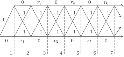
Example 3.12. Let the data be as follows forj1:
Yj= {0, 1}, Sj=
(j, 0), (j, 1), s0=(0, 0),
Yj
sj−1
=Yj(j−1,k)=Yj= {0, 1},
fjsj−1,yj=fj(j−1,k),yj=
j,k+yj, ifk=0,
j,k−yj
, ifk=1,j2.
1 1 1 1 1 1 1 1 1 1 1 1 1 r6 0 r4 0 r2 0 0 r5 0 r3 0 r1 0
[image:14.468.128.342.69.168.2]1 2 3 4 5 6 7
Figure 3.1. State-space diagram forExample 3.12.
To introduce the cost structure, letrk=kj=0(1/2)j, fork=0, 1,..., so thatrk↑2, ask→
∞. Define
cjsj−1,yj=cj(j−1,k),yj=
1, ifyj=0,
0, ifyj=0,j+kis odd,
rj, ifyj=0,j+kis even.
(3.35)
(SeeFigure 3.1.)
Note that the period costs are uniformly bounded. We leave it to the reader to verify that this example has the following properties forα=1, that is, the undiscounted case:
(i)C∗(1)= ∞andA∗(1)=1, which is attained,
(ii)∅ =Xs(1)=Xo(1)⊂ {θ} =Xw(1)=Xe(1)⊂ {x∈X:A(x)=1} =Xa(1)=X,
whereθ=(0, 0,...), so thatXais not contained inXw, in general.
That is, there is exactlyoneefficient optimal solution,noovertaking optimal solution, and allfeasible solutions are average optimal.
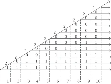
Example 3.13. Let the data be as follows forj1:
Yj= {0, 1}, Sj=
(j, 0), (j, 1),..., (j,j),
s0=(0, 0), Yjsj−1=Yj(j−1,k)= {0},
if 0≤k < j−1, {0, 1}, ifk=j−1,
fjsj−1,yj= fj(j−1,k),yj= (j,k),
if 0≤k≤j−1,yj=0,
(j,k+ 1), ifk=j−1,yj=1.
(3.36)
To introduce the cost structure, define
cj
sj−1,yj
=cj
(j−1,k),yj =
1, if 0≤k < j−1,yj=0,
0, ifk=j−1,yj=0,
2, ifk=j−1,yj=1,
(3.37)
0 0 0 0 0 1 1 1 1 1 0 0 0 0 1 1 1 1 1 0 0 0 0 1 1 1 1 0 0 0 1 1 1 1 0 0 0 1 1 1 0 0 1 1 1 0 0 1 1 0 1 1 0 1 1 2 2 2 2 2 2 2 2 2 2
[image:15.468.120.347.69.241.2]1 2 3 4 5 6 7 8 9 10
Figure 3.2. State-space diagram forExample 3.13.
Note that the period costs are uniformly bounded. We leave it to the reader to verify that this example has the following properties for the undiscounted case:
(i)C∗(1)= ∞andA∗(1)=1, which is attained,
(ii)∅ =Xs(1)⊂ {x0} =Xo(1)=Xw(1)⊂ {xj:j0} =Xa(1)⊂Xe(1)=X, wherexj
is equal to 1 in the firstjpositions and zero thereafter.
That is, there is exactlyone(weakly) overtaking optimal solution, all butoneof the feasible strategies are average optimal, andallfeasible solutions are efficient. Thus,Xwis
properlycontained inXe,Xeisnotcontained inXa, andXaisnotcontained inXw.
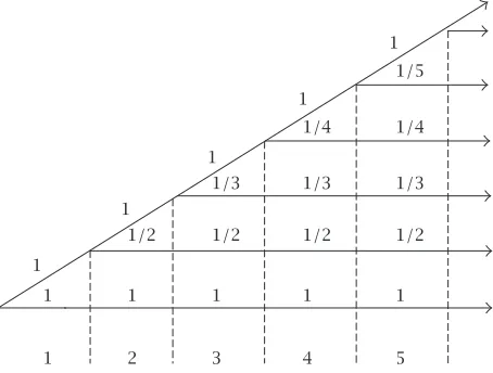
Example 3.14. Let the state-space structure be as in the previous example, but define the cost structure as follows:
cjsj−1,yj=cj(j−1,k),yj= 1
k+ 1, if 0≤k≤j−1, yj=0, 1, ifk=j−1,yj=1,
(3.38)
(seeFigure 3.3.)
Note that the period costs are uniformly bounded. We leave it to the reader to verify that this example has the following properties forα=1, that is, the undiscounted case:
(i)C∗(1)= ∞andA∗(1)=0,
(ii)∅ =Xs(1)=Xo(1)=Xw(1)=Xa(1)⊂Xe(1)=X,
that is,allfeasible strategies are efficient, andnofeasible strategy is optimal in any other sense. Thus,Xw isproperlycontained inXe andXe isnot contained in Xa. Moreover,
1/5
1/4
1/3
1/2
1 1/4
1/3
1/2
1 1/3
1/2
1 1/2
1 1 1 1 1 1 1
[image:16.468.121.348.70.242.2]1 2 3 4 5
Figure 3.3. State-space diagram forExample 3.14.
0 0 0 16 0 0 0 0 0 0 0 8 0 0 0 4 0 2 1 1 1 1 1 1 1 1 1 1 1 1 1 1 1 1 1 1
[image:16.468.124.345.281.358.2]1 2 3 4 5 6 7 8 9 10 11 12 13 14 15 16 17 18
Figure 3.4. State-space diagram forExample 3.15.
Example 3.15. Let the data be as follows forj1:
Yj= {0, 1},
ifj=1,
{0}, ifj >1, Sj=
(j, 0), (j, 1), s0=(0, 0),
Yjsj−1=Yj(j−1,k)= {0, 1},
ifj=1, {0}, ifj2,
fjsj−1,yj=fj(j−1,k),yj=
j,k+yj, ifj=1,
(j,k), ifj2,
cj
sj−1,yj
=cj
(j−1,k),yj =
1, ifj=1,k=0,yj=0,
2, ifj=1,k=0,yj=1,
1, ifj >1,k=0,yj=0,
nj, ifj >1,k=1,yj=0,
(3.39)
wherenj=0, if j+ 1 is not a power of 2, andnj=2m, if j+ 1=2m, for some integer
Note that the period costs are not uniformly bounded, but they are exponentially bounded; specifically, 0≤cj(sj−1,yj)≤2j. Clearly, there are just two feasible solutions
x0andx1, given byx0=(0, 0, 0,...) andx1=(1, 0, 0,...). Moreover, for eachN1, we
haveCN(x0)=Nand
CN
x1=
log2(N+1)
j=1
2j=22log2(N+1)−1, (3.40)
so thatC(x0)= ∞ =C(x1),C∗(1)= ∞, andXs= ∅. For eachN
M=2M−2, we have
CNM
x1=22M−1−1=CNM
x0, ∀M2, (3.41)
that is,CN(x0) andCN(x1) are each equal toN, for all suchN. Next, suppose thatN is
strictly between two such indices, that is, 2M−2< N <2M+1−2, forM2. Then
CNx1−CNx02M+1−2−2M+1−3=1, (3.42)
for suchN. From these facts, it follows that
CN
x1−CN
x00, ∀N, (3.43)
and, in particular, forNM=2M+1−3,
CNM
x1−CNM
x01, ∀M1. (3.44)
Consequently,
lim inf
N
CN
x1−C
N
x00,
lim inf
N
CNx0−CNx1≤ −1,
lim sup
N
CN
x0−CN
x10,
(3.45)
that is,x0overtakesx1(so thatx0weakly overtakesx1),x1does not overtakex0, andx1
weakly overtakesx0. Hence,Xo(1)= {x0}andXw=X. Clearly,Xe(1)=Xalso since, for
each state, only one of the strategies attains that state.
As we have observed, for eachN2, there exists a uniqueM2 such that 2M−2<
N≤2M+1−2, andC
N(x1)=2M+1−2, so that
CNx1
2M+1−2≤
CNx1
N ≤
CNx1
Consequently,
Ax1=lim sup
N
CN
x1
N =Mlim→∞
2M+1−2
2M−1 =2. (3.47)
Thus,C∗(1)= ∞,A∗(1)=1 andXa(1)= {x0}, since clearlyA(x0)=1.
We thus obtain the following inclusions:
∅ =Xs(1)⊂ {x0} =Xo(1)=Xa(1)⊂Xw(1)=Xe(1)=X, (3.48)
so that, in particular,XwandXearenotcontained inXa. There is exactlyoneovertaking
(average) optimal solution,nostrongly optimal solutions, andallfeasible solutions are weakly overtaking and efficient.
Remark 3.16. Example 3.14shows that there exist problems for which our five optimality criteria are indiscriminate. In such cases, other criteria are called for, of which there are many. See Carlson et al. [6], for example.
4. Reachability conditions
In this section, we consider certain additional state-reachability conditions for our prob-lem which will prove to be useful for comparing our optimality criteria in the caseC∗(α) = ∞. These conditions arecontrollabilitynotions. A very strong version of such a notion in the literature iscomplete reachability, which requires that the system be able to transi-tion from any state in any period to any state in the very next period. This was assumed in Zaslavski [22], and most notably in [6, Section 5.3]. Another strong controllability no-tion (used in [14]) requires that transition from any state at any time to any future state be accomplished by a feasiblestationarystrategy. Our state-reachability conditions are considerably weaker than these.
First, we recall (a slightly weaker version of) thebounded reachabilitycondition intro-duced in [18].
Bounded time reachability (BTR). There exists a positive integer Rsuch that for each 1≤K <∞and eachx,y∈X, there existK≤L≤K+Randz∈XL(depending onK,x,
y) for whichsK(z)=sK(y) andsL(z)=sL(x). If suchRexists, then our problem is said
to satisfy thebounded time reachability, that is, property (BTR). Roughly speaking, there exists a strategyzwhich steers the system from statesK(y) at timeKto statesL(x) at some
timeL, which is at mostRperiods fromK.
Note that property BTR is independent of the cost structure and the discount factor. Consequently, we introduce two other notions of state-reachability which do depend on these data.
Total cost reachability (TCR|α). Let x,y∈X, 0< α≤1. For each >0, there exists a positive integerM(depending on), such that for allNM, there exist 0≤K≤Nand z∈X(depending onN) such thatsK(z)=sK(y),sN(z)=sN(x) andCN(z|α)−CK(z|α)<
Average cost reachability (ACR|α). Letx,y∈X. Given>0, there exists a positive integer M such that for allNM, there exists 0≤K≤N andz∈X such thatsK(z)=sK(y),
sN(z)=sN(x) andCN(z|α)−CK(z|α)< N. Thus, here steering is as in the previous case,
but with average cost less than.
Obviously, these reachability properties do depend on the cost structure and the dis-count factor. Moreover, the average cost reachability property is weaker than the total cost reachability property, that is, (TCR|α)⇒(ACR|α), for all 0< α≤1. The converse is false, in general (Example 4.5).
Ifcj are exponentially bounded, say byBeγ j, andα <1/γ, then strong optima exist
(Section 3), and they are optimal in every other sense. However, ifα1/γorcjare not
exponentially bounded, then what can we say? The next result sets the stage for our re-sponse to this question, which depends on the relationship betweenαandcj.
Theorem4.1. Suppose property BTR holds. (i)Ifαis such that
lim
j→∞ αj−1c
j
j =0, (4.1)
then property (ACR|α) holds. In particular, if
lim
j→∞ cj
j =0, (4.2)
then property (ACR|α) holds for all0< α≤1. (ii)Ifαis such that
lim
j→∞α j−1
cj=0, (4.3)
then property (TCR|α) holds. In particular, if
lim
j→∞ c
j=0, (4.4)
then property (TCR|α) holds for all0< α≤1.
Proof. (i) LetR1 be as property BTR. Givenx,y∈X and>0, letJ be sufficiently large such that
αj−1c
j
j <
R, ∀jJ. (4.5)
LetM=J+RandNM. SetK=N−RJ. By property BTR, there existsLsuch that
andw∈XLsuch thatsK(w)=sK(y) andsL(w)=sL(x). Letz=(w|Lx) so thatsK(z)=
sK(w)=sK(y) andsN(z)=sN(x). Also,
CN(z|α)−CK(z|α)= N
j=K+1
αj−1cj
sj−1(z),zj
≤ N
j=K+1
αj−1c
j≤
R
N
j=K+1
j
≤N(N−K) R=N.
(4.7)
Thus, property (ACR|α) holds. Part (ii) is proved similarly.
Remark 4.2. It is worth noting that, for each 0< α≤1, it can happen that the hypotheses ofTheorem 4.1hold, together with the property thatC∗(α)= ∞. For example, it happens whenα=1 andcj =B/ j.
In Schochetman and Smith [18, Theorem 4.2], we showed that, in the presence of property BTR, every efficient strategy is average optimal, that is,Xe(α)⊆Xa(α), for all
0< α≤1. We next give a stronger version of this result. Thus, we obtain reasonable suf-ficient conditions for the existence of average optima—which need not exist in general (Example 3.15). Note that ifA∗(α)= ∞, thenXa(α)= ∅, for suchα, and, at least in the
discrete case,Xe(α) can’t possibly be contained therein, since it is nonempty.
Theorem4.3. Supposeαis such that property (ACR|α) is satisfied andA∗(α)<∞. Then efficient implies average optimal, that is,Xe(α)⊆Xa(α), so that
Xs(α)⊆Xo(α)⊆Xw(α)⊆Xe(α)⊆Xa(α), (4.8)
for suchα. If, in addition, the set-valued functionssXN(s)are continuous, then there
exists an efficient optimum which is also average optimal.
Proof. Letx∈Xe(α), and suppose there existsy∈Xsuch thatA(y|α)< A(x|α), that is,
x /∈Xa(α). In particular,A(y|α)<∞. Let
= 1 2
A(x|α)−A(y|α), ifA(x|α)<∞,
1, ifA(x|α)= ∞, (4.9)
so that>0. Also letMbe as in property (ACR|α) forx,yand. Then, for eachNM, there exist 0≤K≤N andz∈Xsuch thatsK(z)=sK(y),sN(z)=sN(x), andCN(z|α)−
CK(z|α)< N. IfK=N, thenz=y,sN(z)=sN(x)=sN(y), andCN(y|α)CN(x|α), that
IfK < N, definew=(y|Kz), so thatw∈XandsN(w)=sN(z) byLemma 2.3. Then,
necessarily,CN(x|α)≤CN(w|α), sincex∈Xe(α) andw∈XwithsN(w)=sN(x).
More-over,CN(y|α)CK(y|α), since eachcj0. Thus,
CN(y|α) + N
j=K+1
αj−1c
j
sj−1(z),zj
CK(y|α) + N
j=K+1
αj−1c
j
sj−1(z),zj
=CK(w|α) +CN(w|α)−CK(w|α)
=CN(w|α)
CN(x|α)
=N
j=1
αj−1c
j
sj−1(x),xj
,
(4.10)
which implies that
1
NCN(y|α) + 1 N
N
j=K+1
αj−1c
jsj−1(z),zj 1
N
N
j=1
αj−1c
jsj−1(x),xj, (4.11)
that is,
AN(y|α) + 1
N
CN(z|α)−CK(z|α)AN(x|α). (4.12)
SinceCN(z|α)−CK(z|α)< N, we have that
AN(y|α) +> AN(y|α) +N1
CN(z|α)−CK(z|α)
AN(x|α), (4.13)
for the caseK < N. Thus,AN(y|α) +> AN(x|α), for allNM. Consequently,
lim sup
N AN(y|α) +=
lim sup
N
AN(y|α) +
=lim sup
NM
AN(y|α) +
lim sup
NM
AN(x|α)
=lim sup
N AN(x|α),
(4.14)
Theorem4.4. Ifαis such that property (TCR|α) is satisfied, then every efficient strategy is overtaking optimal, that is,Xe(α)⊆Xo(α), so that
Xs(α)⊆Xo(α)=Xw(α)=Xe(α). (4.15)
If, in addition,A∗(α)<∞, then
Xs(α)⊆Xo(α)=Xw(α)=Xe(α)⊆Xa(α). (4.16)
Proof. ByCorollary 3.7, it suffices to show the set inclusion for the first claim. Fixx∈ Xe(α) and lety∈X. We show thatxovertakesy. Let>0. By property (TCR|α), there
exists a positive integer M such that for all NM, there exist 0≤K≤N and z∈X such thatsK(z)=sK(y),sN(z)=sN(x), andCN(z|α)−CK(z|α)<. Letw=(y|Kz). Then
w∈X,sK(w)=sK(y),sN(w)=sN(z)=sN(x), and
CN(w|α)−CK(w|α)=CN(z|α)−CK(z|α)<. (4.17)
Hence, by the efficiency ofxat horizonN, we have
CN(x|α)≤CN(w|α)=CK(w|α) +CN(w|α)−CK(w|α)
< CK(y|α) +
≤CN(y|α) +.
(4.18)
Therefore,x∈Xo(α). To complete the proof, applyTheorem 4.3, together with the fact
that (TCR|α)⇒(ACR|α).
Example 4.5. Let the data be as inExample 3.12. We leave it to the reader to verify that this example has properties BTR withR=1, (ACR|α), for all 0< α≤1, and (TCR|α), for all 0< α <1, that is, it doesnothave property (TCR|1).
Examples 4.6. Let the data be as in Examples3.13,3.14, or3.15. We leave it to the reader to verify that, for each example, and for each 0< α≤1, all three reachability properties fail.
Before leaving this section, we summarize our main results.
Theorem4.7. The following are true for our general optimization problem.
(i)If the set-valued mappingssXN(s)are continuous, thenXe(α)= ∅, that is, efficient
optima exist, for each0< α≤1. (ii)IfC∗(α)= ∞, thenXs(α)= ∅.
(iii)IfC∗(α)<∞, then it is attained,A∗(α)<∞, and
∅ =Xs(α)⊆Xo(α)⊆ X
w(α)⊆Xe(α),
Xa(α), (4.19)
so that there exists a strong optimum which is optimal in every sense. (iv)IfA∗(α)= ∞, thenC∗(α)= ∞,Xs(α)=Xa(α)= ∅, and
(v)IfA∗(α)<∞, then
∅ ⊆Xs(α)⊆Xo(α)⊆ X
w(α)⊆Xe(α),
Xa(α). (4.21)
(vi)IfA∗(α)<∞and property (ACR|α) holds, then
Xs(α)⊆Xo(α)⊆Xw(α)⊆Xe(α)⊆Xa(α), (4.22)
and, in particular, efficient optima are average optimal. (vii)IfA∗(α)<∞and property (TCR|α) holds, then
Xs(α)⊆Xo(α)=Xw(α)=Xe(α)⊆Xa(α), (4.23)
and, in particular, efficient optima are overtaking, weakly overtaking, and average optimal.
Acknowledgment
The first author was supported in part by an Oakland University Research Fellowship. The second author was supported in part by the National Science Foundation under Grants DMI-9713723 and DMI-0322114.
References
[1] A. Arapostathis, V. S. Borkar, E. Fern´andez-Gaucherand, M. K. Ghosh, and S. I. Marcus,
Discrete-time controlled Markov processes with average cost criterion: a survey, SIAM J. Con-trol Optim.31(1993), no. 2, 282–344.
[2] D. P. Bertsekas,Dynamic Programming: Deterministic and Stochastic Models, Prentice Hall, New Jersey, 1987.
[3] ,Dynamic Programming and Optimal Control, Vol. 1 and 2, Athena Scientific, Mas-sachusetts, 1995.
[4] W. A. Brock,On existence of weakly maximal programmes in a multi-sector economy, Rev. Econom. Stud.37(1970), no. 2, 275–280.
[5] W. A. Brock and A. Haurie,On existence of overtaking optimal trajectories over an infinite time horizon, Math. Oper. Res.1(1976), no. 4, 337–346.
[6] D. A. Carlson, A. Haurie, and A. Leizarowitz,Infinite Horizon Optimal Control. Deterministic and Stochastic Systems, 2nd ed., Springer, New York, 1991.
[7] G. Chichilnisky,Sustainable development and social choice, Paine-Webber Working Paper Series in Money, Economics and FinancePW-94-02(1993), 1–20.
[8] R. R. Goldberg,Methods of Real Analysis, Blaisdell, Waltham, 1964.
[9] H. Halkin,Necessary conditions for optimal control problems with infinite horizons, Economet-rica42(1974), 267–272.
[10] A. Haurie,Optimal control on an infinite time horizon: the turnpike approach, J. Math. Econom.
3(1976), no. 1, 81–102.
[11] E. Hewitt and K. Stromberg,Real and Abstract Analysis. A Modern Treatment of the Theory of Functions of a Real Variable, Springer, New York, 1965.
[13] ,Decision horizon, overtaking and1-optimality criteria in optimal control, Advances in Optimization and Control (Montreal, PQ, 1986) (H. A. Eiselt and G. Pederzoli, eds.), Lec-ture Notes in Econom. and Math. Systems, vol. 302, Springer, Berlin, 1988, pp. 247–261. [14] A. Leizarowitz,Infinite horizon optimization for finite state Markov chain, SIAM J. Control
Op-tim.25(1987), no. 6, 1601–1618.
[15] ,Overtaking and almost-sure optimality for infinite horizon Markov decision processes, Math. Oper. Res.21(1996), no. 1, 158–181.
[16] S. M. Ryan, J. C. Bean, and R. L. Smith,A tie-breaking rule for discrete infinite horizon optimiza-tion, Oper. Res.40(1992), no. suppl. 1, S117–S126.
[17] I. E. Schochetman and R. L. Smith,Finite-dimensional approximation in infinite-dimensional mathematical programming, Math. Program.54(1992), no. 3, 307–333.
[18] ,Existence and discovery of average optimal solutions in deterministic infinite horizon optimization, Math. Oper. Res.23(1998), no. 2, 416–432.
[19] A. F. Veinott Jr.,On finding optimal policies in discrete dynamic programming with no discount-ing, Ann. Math. Statist.37(1966), 1284–1294.
[20] C. C. Von Weiszacker,Existence of optimal programs of accumulation for an infinite time horizon, Rev. Econom. Stud.32(1965), 85–104.
[21] D. V. Widder,The Laplace Transform, Oxford University Press, Oxford, 1946.
[22] A. J. Zaslavski,Optimal programs on infinite horizon. I, II, SIAM J. Control Optim.33(1995), no. 6, 1643–1686.
Irwin E. Schochetman: Department of Mathematics and Statistics, Oakland University, Rochester, MI 48309, USA
E-mail address:[email protected]
Robert L. Smith: Department of Industrial and Operations Engineering, The University of Michi-gan, Ann Arbor, MI 48109, USA