Dynamics and Thresholds of a Simple Epidemiological Model: Example of HIV/AIDS in Mali

(1)

Volume 2010, Article ID 638021,8pages doi:10.1155/2010/638021

Research Article

Dynamics and Thresholds of

a Simple Epidemiological Model:

Example of HIV/AIDS in Mali

Ouat ´eni Diallo,

1

_{Yaya Kon ´e,}

1

_{and J ´er ˆome Pousin}

2

1_{Département de Mathématiques et D’Informatique, Faculté des Sciences et Techniques,}

B.P.E 3206, Bamako, Mali

2_{Universit´e de Lyon, INSA, ICJ UMR CNRS 5208, 69100 Lyon, France}

Correspondence should be addressed to J´er ˆome Pousin,[email protected]

Received 23 March 2010; Revised 13 August 2010; Accepted 23 September 2010

Academic Editor: Thomas Witelski

Copyrightq2010 Ouat´eni Diallo et al. This is an open access article distributed under the Creative Commons Attribution License, which permits unrestricted use, distribution, and reproduction in any medium, provided the original work is properly cited.

The dynamics of many epidemiological models for infectious diseases that spread in the sexually active population presents a crucial period: the period of the influx or recruitment of susceptible. In this paper, we assume that the recruitment of susceptible is done among the juvenile group. We propose a dynamical system to modelize the disease spread, and we study the dynamical behavior of this system. Then, the controllability of the system is studied. We prove that the survival rate allows to control the dynamic of the system. Numerical simulations are given to illustrate the results.

1. Introduction

In recent years several authors have described interesting dynamical behavior of SIR epidemiological models in which the population can be portioned into two age structured classes: immature individuals and mature onessee, e.g.,1,2. The HIV disease belongs to the class of diseases which spread essentially among sexually active individuals. Thus, it is meaningful to consider stage structure in epidemiological models. The population is initially divided into two compartments: those, who are mature individuals or adults and those who are in youthful age or immature individuals. All population groups are subject to the risk of dying from AIDS.

We denote by

iBthe birth density in the population;

(2)

iiiMthe density of the mature individuals;

ivNthe density of the population;

vDthe density of the dead individuals;

vidthe probability of mature individuals to die of HIV;

viimthe probability of immature individuals becoming mature individuals;

viiinthe probability of mature individuals to die of other causes.

Then a simple model with compartments and a single population with stage structure reads:

N B J m M

d n

D

1.1

NJN 1.2

For describing the disease transmission, a dynamics between the compartments due to the disease has to be specified. A traditional SIR model is introduced. Each member of the population is considered to belong to one of the three classes: susceptible individuals

denoted byS, infected individualsdenoted byIand removed individualsdenoted by

R. Each individual begins in the classS, only to move to the classIafter coming into contact with an infected person. Infected individuals eventually recover from the disease due to a medical treatment and then move to the classRand are unable to be infected one again. The disease is fueled by supply of susceptible issued from the compartmentJ. The size of the population is denoted byNtand can be expressed as the following sum:

Nt St It Rt Jt. 1.3

The SIR model reads

dS

dt r1m1−τJt−FiI, tSr2S, dI

dt FiI, tS−r3σαI, dR

dt r3σI−μR,

1.4

where FiI, tis the incidence function which may vary periodically because a part of the infected population represented by the truck drivers, for example, moves regularly. It is usual to takeFiI, t ΩtIin whichΩtis the transmission rate; it is either constant, or a periodic modulation about a constant value, for example,Ωt Ω01 Ω1sinωt;mis the rate of

immature individuals becoming mature individuals;r1 is the survival rate of the immature

individuals; r2 is the survival rate of the mature individuals;r3 is the survival rate of the

(3)

The aim of this work is to provide simple conditions for the parameters of the SIR model1.4that makes possible to control the infected individuals. By using the notion of the exterior contingent cone to a convex subsetCofR2_{, we prove that system}_1.4_{is controllable}

with three of its parameters. Whatever the initial conditions are, system 1.4 reaches the subsetCand remains inC. The paper is organized as follows: the introduction ends with an existence and uniqueness result. InSection 2the controllability of system1.4is studied and several numerical results are presented in connection with available data concerning Mali.

The dynamic behavior of1.4is determined by the variation ofIandR. According to

1.3the susceptible compartment is expressed asSt Nt−It−Rt−Jt, thus1.4is reduced to

dI

dt FiI, tNt−Jt−Rt−It−r3σαI, dR

dt r3σI−μR.

1.5

Sinceμ >0, a new timescaletμtis introduced. System1.5becomes:

dI dt Ω

tIN−J−R−I−r₃σαI,

dR dt r

3σI−R.

1.6

We assume thatΔ Nt−Jt−Rtis constant. Definingγ r₃σ, and omitting the prime notations, system1.6becomes:

dI

dt ΩtIΔ−I−γI− γα

σ I,

dR

dt γI−R.

1.7

Theorem 1.1. Assumes that Ωis a C1_R

;Rfunction with bounded primitive. For every initial conditionI∗, R∗ ∈ R2, the solutionI·, R· : R → R2 of 1.7belongs toKwhere Kis a compact subset ofR2

.

Proof. Setθγ1α/σ, by integrating the first equation of1.7we have

It I0e

t

0ΩτΔ−θdτ 1₀tI0e

t

0ΩτΔ−θdτ ds

. 1.8

LetMbe a bound from below of a primitive ofΩ, the we have

0≤It< I0e

MΔt

eθt₁t

0I0e

t

0ΩτΔ−θdτ ds

(4)

FromdR/dtγI−Rwe deduce

Rt R0e−tγe−t

t

0

es_I_s_ds

≤R0e−tγe−t

et−1I

< R0e−tγIR.

1.10

So the Poincar´e-Bendixson’s theorem3claims either the solution I, R of system

1.7tends to a critical point when the timetgoes to infinity, or it is a periodic solution. A complete bifurcation analysis is beyond the objectives of this paper. For a precise study of the orbits the reader is referred to4or5, for example.

2. Controllbility of the Model with Its Coefficients

The question we address in this section reads: does there exist parameters which allow system

1.7to evolve toward a fixed regionCof the planeI, R, for any given initial condition? For 0< x₁fixed, we define the convex domainCof the plane and its associated truncated cylinder

CTby:

C

x1, x2∈R2; x1≤x₁; and

3

4x1≤x2 ,

CT

t, x1, x2∈R3; 0≤t≤T; x1≤x₁; and

3

4x1 ≤x2 .

2.1

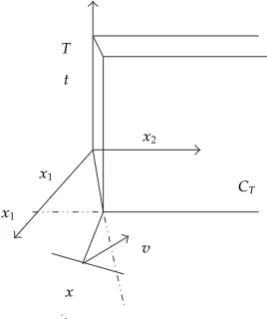
Definition 2.1contingent and exterior contingent cone. The contingent cone toCTatxTCTx is constituted by vectorsv∈R3_verifying

lim h→0inf

dCTxhv, CT

h 0, 2.2

where dCT denotes the distance to the subset CT. The exterior contingent cone TCTx is constituted by vectorsv∈R3_verifying

lim h→0inf

dCTxhv, CT−dCTx

h ≤0. 2.3

When a pointx belongs to the boundary ofCT the definition of exterior contingent cone is equivalent to the definition of the contingent cone. We have the following result6, Theorem 3.4.1 page 102.

Lemma 2.2. The exterior contingent cone toCTat pointxis constituted by vectorsv∈R3satisfying:

x−PCTx, v≤0; 2.4

(5)

Before stating the result of controllability, we give some technicalities. Setting

Ft, x1, x2

⎛ ⎜ ⎜ ⎝

1

Ωtx1Δ−x1−x1γ

1α

σ

γx1−x2

⎞ ⎟ ⎟

⎠, 2.5

we have the following.

Lemma 2.3. LetX ∈ {t, x1, x2, 0< t < T; 0 < x1; 0< x2} ∩C_Tc be fixed. ThenX−PCTXis the

outward normal toCT whenever it exists, and for 0≤s≤1 is given by

X−PCTX

⎛ ⎜ ⎜ ⎝ 0 1 −4 3s ⎞ ⎟ ⎟

⎠. 2.6

Furthermore, a suﬃcient condition for the vectorFXto belong to the exterior contingent coneTCT

read as follows:

x1

ΩtΔ−x1−γ

1 α

σ

1

≤0. 2.7

Proof. From the definition of the exterior contingent coneFigure 1TCT we have:

∀s∈0,1, −Ωtx2 1x1

ΩtΔ−γ

1α

σ

−4s 3

≤ 4s

3 x2. 2.8

A suﬃcient condition independent ofsfor condition2.8to be satisfied is obtained when

x2≤3/4x1with 0≤x1and read as follows:

−Ωtx2₁x1

ΩtΔ−γ

1 α

σ

≤ −x1. 2.9

Theorem 2.4. Let 0 ≤ max0≤tΩt Ω, and let parametersα, 0 < x1 < Δ,σbe fixed. Whatever

I0, R0∈R2are, chooser₃ in such a way thatγr₃σverifies:

0<

γ−3

4

; ΩΔ−x₁−γ

1α

σ

1≤0. 2.10

Then, there exists 0≤Trsuch that for all timet≥Tr, the solutionIt, Rtof problem1.7belongs

(6)

v

x x1

x1

CT t

T

[image:6.600.232.366.98.258.2]

x2

Figure 1: Exterior contingent cone.

Proof. SetY t, It, Rt, then problem1.7 is expressed as the following autonomous system:

dYt

dt FYt; 0< t, Y0 0, I0, R0.

2.11

Define the functionGt, Iby

Gt, I ΩtΔ−I−γ

1 α

σ

1. 2.12

FunctionGis a decreasing function with respect toIfor all time. Thus ifGt, x1≤0, it will

be negative for allI > x1. Condition2.10implies thatF2t, I, Ris negative andF3t, I, R

is positive for all 0< t;x1 < I; 0≤ R.Theorem 1.1asserts the existence ofIt, Rtfor all

timet. A simple continuity argument implies that the subsetCdefined in2.1is reached for a time Tr by the trajectory starting at the point I0, R0. FixT > Tr,Lemma 2.2claims that condition2.10is suﬃcient forFY∈ TCTYwhenY belongs to the boundary ofCT. Nagumo’s theorem applies for equation2.11with initial conditions Tr, Itr, RTr, and we getIt, Rt∈CforTr ≤t7, Theorem 1, page 27.

As consequence of Theorem 2.4 the SIR models allow to improve the efficiency of medical policies. The sufficient condition 2.10characterizes the treatment effort through the survival rater3of the infected mature individuals recovered with the rateσ.

Let us end this section with numerical examples. The system1.7is discretized with a Runge-Kutta’s methodRK4. By using available data from Mali in system1.7we have the following values for parameters:Δ 6066573;γ 0.25;α0.01;x₁ 1.5 105_{. The following}

(7)

0.5 1 1.5 2 2.5 3 3.5 4 4.5 5 5.5

×105

×104

2 3 4 5 6 7 8 9 10 11

R

Trajectory of system(1.6)

I a

1 2 3 4 5 6 7 8 9 10

×105

0.4 0.6 0.8 1 1.2 1.4 1.6 1.8

×105 Trajectory of system(1.6)

I R

[image:7.600.110.488.100.280.2]

b

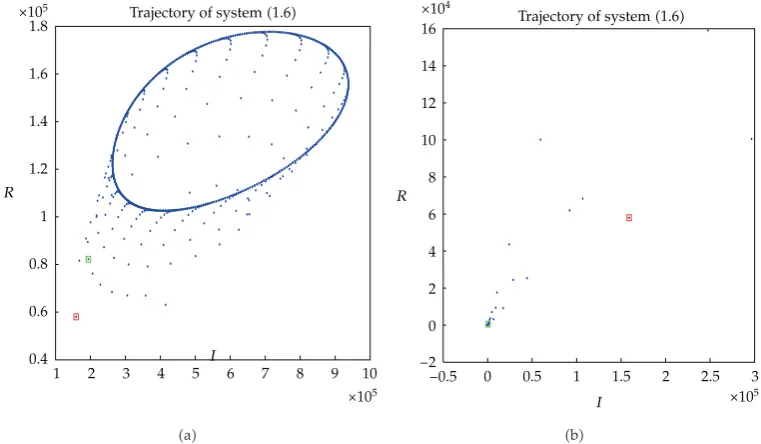
Figure 2:a ΩΔ−x₁−γ1α/σ≤ −1,b ΩΔ−x₁−γ1α/σ 1>0.

I R

1 2 3 4 5 6 7 8 9 10

×105

0.4 0.6 0.8 1 1.2 1.4 1.6 1.8

a

−0.5 0 0.5 1 1.5 2 2.5 3 ×105 −2

0 2 4 6 8 10 12 14 16 ×104

R

I

b

Figure 3:a 3/4x1≤x2is not satisfied withr30.85;b 3/4x1≤x2is satisfied withr32.

The initial conditions areI0, R0 1.59 105,5.8 104 denoted by the red point. InFigure 2

we have considered the caseawithΩ 4.3 10−8_;_σ ₀_._{5. The su}_ﬃ_{cient condition}_2.10

is not satisfied, nevertheless, it can be checked that after a long time the computed solution

It, Rthas a first component less than or equal tox1. In caseb, we haveΩ 4.6 10−8; σ0.8. The suﬃcient condition2.10is not satisfied. Here the trajectory is outside the cone

CT.

[image:7.600.109.490.325.547.2]

(8)

the survival rater3of the infected mature individuals recovered at a rateσ. In the following

examples, keeping the same values for parameters as in caseaexcept forr3. Forr3 0.85,

The suﬃcient condition 2.10 is not satisfied, and we have in Figure 3a the trajectory outside CT. For r3 2, the suﬃcient condition 2.10 is satisfied, and the trajectory is

concentrated in a neighborhood of the disease-free equilibrium0,0seeFigure 3b.

3. Conclusion

In this paper, it is shown by using the exterior contingent cone and a viability theorem, simple convex subsets are reachable with a SIR model by adjusting some coeﬃcients. Thus, it will be possible to predict with a certain accuracy the evolution level of the disease by adjusting one or another of parameters. In our example, it is important to see that, if the survival rater3 attains 2%, the disease almost goes back at a level disease-free equilibrium.

The controllability of the dynamical system has been established by using the exterior contingent cone technique. The mathematical model could be improved by introducing new compartments for describing, for example, the transmission of the disease between mothers and children. If the exterior contingent cone, for ordinary diﬀerential system of higher dimension, can be defined in the same way as before, it has to be calculable that which is an open question in general.

References

1 W. R. Derrick and P. van den Driessche, “Homoclinic orbits in a disease transmission model with nonlinear incidence and nonconstant population,” Discrete and Continuous Dynamical Systems. Series B, vol. 3, no. 2, pp. 299–309, 2003.

2 X. Li and W. Wang, “A discrete epidemic model with stage structure,” Chaos, Solitons and Fractals, vol. 26, no. 3, pp. 947–958, 2005.

3 J. Guckenheimer and P. Holmes, Nonlinear Oscillations, Dynamical Systems, and Difurcations of Vector

Fields, vol. 42 of Applied Mathematical Sciences, Springer, New York, NY, USA, 1983.

4 G.-J. Han, “Bifurcation analysis on an unfolding of the Takens-Bogdanov singularity,” Journal of the

Korean Mathematical Society, vol. 36, no. 3, pp. 459–467, 1999.

5 C. Wolf, Mod´elisation et analyse math´ematique de la propagation d’un micro-parasite dans une population

structurée en environnement hétérogène, Thèse de doctorat, 2005.

6 M. Picq, Résolution de l’équation du transport sous contraintes, Thèse de Doctorat, Institut National des Sciences Appliquées INSA de Lyon, Lyon, France, 2007, http://docinsa.insa-lyon.fr/these/pont .php?&idpicq.