MKM227 Postgraduate Dissertation
Comments Max
Mark
Actual Mark
Introduction
Identification of a valid topic, research question and
objectives framed to Masters Level standard with academic rationale developed, clear industry contextualisation of the research topic
Supervisor Comments:
10%
2nd marker Comments:
Critical Literature Review Depth and breadth of
Supervisor Comments:
2 | U 1 0 4 3 8 5 3 literature search, engagement
with seminal authors and papers, evidence of a critical approach toward the scholarly literature
2nd marker Comments:
Research Methodology Evaluation of research
philosophies and perspectives. Justification of methodological approach, sampling strategy, data analysis and reliability and validity measures as applicable
Supervisor Comments:
15%
2nd marker Comments:
Supervisor Comments:
3 | U 1 0 4 3 8 5 3 Data Analysis and
Interpretation
Evidence of rigor in data analysis and interpretation procedures, identification of key patterns and themes in the research data, integration of academic theory into
explanation of findings
2nd marker Comments:
Conclusions and Recommendations Research question and objectives addressed with implications to theoretical and managerial concepts
considered. Recommendations provided for theory, practice and future research
Supervisor Comments:
10%
4 | U 1 0 4 3 8 5 3 Organisation, presentation
and references.
Well structured and ordered dissertation with correct use of grammar and syntax. In-text citation and bibliography
Supervisor Comments:
5%
2nd marker Comments:
Total
First Marker Total
100%
5 | U 1 0 4 3 8 5 3
Supervisor General Comments: Agreed Mark:
2nd Marker General Comments:
6 | U 1 0 4 3 8 5 3
[Modelling the Frequency of Operational Risk Losses under the Basel II
Capital Accord:
A Comparative study of Poisson and Negative Binomial Distributions]
A dissertation submitted in partial fulfilment of the requirements of the Royal Docks Business School, University of East London for the degree of
[Master in Science in RISK MANAGEMENT]
[September, 2013]
[15,873]
I declare that no material contained in the thesis has been used in any other submission for an academic award
Student Number: U1043853 Date: 2nd September 2013
7 | U 1 0 4 3 8 5 3 Libraries and Learning Services at UEL is compiling a collection of
dissertations identified by academic staff as being of high quality. These dissertations will be included on ROAR the UEL Institutional Repository as examples for other students following the same courses in the future, and as a showcase of the best student work produced at UEL.
This Agreement details the permission we seek from you as the author to make your dissertation available. It allows UEL to add it to ROAR and make it available to others. You can choose whether you only want the
I DECLARE AS FOLLOWS:
That I am the author and owner of the copyright in the Work and grant the University of East London a licence to make available the Work in digitised format through the Institutional Repository for the purposes of non-commercial research, private study, criticism, review and news reporting, illustration for teaching, and/or other educational purposes in electronic or print form
That if my dissertation does include any substantial subsidiary material owned by third-party copyright holders, I have sought and obtained permission to include it in any version of my Work available in digital format via a stand-alone device or a communications network and that this permission encompasses the rights that I have granted to the University of East London.
That I grant a non-exclusive licence to the University of East London and the user of the Work through this agreement. I retain all rights in the Work including my moral right to be identified as the author. That I agree for a relevant academic to nominate my Work for adding to ROAR if it meets their criteria for inclusion, but understand that only a few dissertations are selected.
That if the repository administrators encounter problems with any digital file I supply, the administrators may change the format of the file. I also agree that the Institutional Repository administrators may, without changing content, migrate the Work to any medium or format for the purpose of future preservation and accessibility.
That I have exercised reasonable care to ensure that the Work is original, and does not to the best of my knowledge break any UK law, infringe any third party's copyright or other Intellectual Property Right, or contain any confidential material.
8 | U 1 0 4 3 8 5 3 breach of contract or of any other right, in the Work.
I FURTHER DECLARE:
anyone worldwide using ROAR without barriers and that files will also be available to automated agents, and may be searched and copied by text mining and plagiarism detection software.
That if I do not choose the Open Access option, the Work will only be available for use by accredited UEL staff and students for a limited period of time.
9 | U 1 0 4 3 8 5 3 Dissertation Details
Field Name Details to complete
Title of thesis
Full title, including any subtitle
Modelling the Frequency of Operational
Risk Losses under the Basel II Capital
Accord:
A Comparative study of Poisson and Negative Binomial Distributions Author
Separate the surname (family name) from the forenames, given names or initials with a comma, e.g. Smith, Andrew J.
SILVER, Toni O.
Supervisor(s)/advisor Format as for author.
CHAN, Tat Lung (Ron)
Author Affiliation
Name of school where you were based
University of East London
Qualification name
E.g. MA, MSc, MRes, PGDip
MSc
Course Title
The title of the course e.g.
MSc Risk Management
Date of Dissertation
Date submitted in format: YYYY-MM
2013-09
Do you want to make the
dissertation Open Access (on the public web) or Closed Access (for UEL users only)?
Open Closed
By returning this form electronically from a recognised UEL email address or UEL network system, I grant UEL the deposit agreement detailed above. I understand inclusion on and removal from ROAR is at
10 | U 1 0 4 3 8 5 3 Name: Toni O Silver
11 | U 1 0 4 3 8 5 3
Modelling the Frequency of Operational Risk Losses under the
Basel II Capital Accord:
A Comparative study of Poisson and Negative Binomial Distributions
Dissertation submitted as part of the requirements of the degree of
MASTER IN SCIENCE IN RISK MANAGEMENT,
UNIVERSITY OF EAST LONDON
By
Toni Silver - U1043853
September, 2013
12 | U 1 0 4 3 8 5 3 TABLE OF CONTENT
ABSTRACT ... 14
ACKNOWLEDGEMENTS ... 16
CHAPTER ONE ... 16
1. INTRODUCTION ... 16
1.1 POISSON AND NEGATIVE BINOMIAL DISTRIBUTIONS ... 18
1.2 PURPOSE OF THE STUDY ... 18
1.3 RATIONALE OF THE STUDY ... 19
1.4 RESEARCH QUESTIONS ... 20
1.5 SIGNIFICANCE OF THE STUDY ... 21
CHAPTER TWO ... 21
2. REVIEW OF LITERATURE... 21
2.1 WHAT CONSTITUTES OPERATIONAL RISK ... 22
2.2 CLASSIFICATION OF OPERATIONAL RISK ... 23
2.2.1 THE BASEL II CAPITAL ACCORD ... 24
2.2.2 ADVANCED MEASUREMENT APPROACH ... 26
2.2.2.1 THE LOSS DISTRIBUTION APPROACHES ... 27
2.3 FREQUENCY AND SEVERITY DISTRIBUTIONS ... 29
2.3.1 FREQUENCY DISTRIBUTIONS ... 30
2.3.1.1 THE BINOMIAL DISTRIBUTION ... 31
2.3.1.2 THE GEOMETRIC DISTRIBUTION ... 32
2.4 POISSON DISTRIBUTION ... 32
2.4.1 WHY CHOOSE THE POISSON DISTRIBUTION ... 33
2.5 NEGATIVE BINOMIAL DISTRIBUTION ... 34
2.5.1 WHY CHOOSE THE NEGATIVE BINOMIAL ... 35
2.6 EMPIRICAL STUDIES ON POISSON AND NEGATIVE BINOMIAL ... 36
2.7 SUMMARY OF CHAPTER ... 37
CHAPTER THREE ... 38
3. RESEARCH METHODOLOGY ... 38
3.1 POPULATION AND SAMPLING ... 39
3.2 VALIDITY AND RELIABILITY OF INSTRUMENTS ... 39
3.3 DATA COLLECTION ... 40
3.4 DATA ANALYSIS ... 41
13 | U 1 0 4 3 8 5 3
3.4.1.1. ... 42
3.4.1.2 HYPOTHESES TESTING ... 42
3.5 ETHICAL CONSIDERATION ... 43
3.6 LIMITATION OF STUDY ... 43
CHAPTER FOUR ... 44
4. DATA ANALYSIS ... 44
4.1 GROUPED FREQUENCY OF LOSS EVENTS... 45
4.1.1 FREQUENCY OF LOSSES BY BUSINESS LINE/ EVENT TYPE ... 46
4.2 DISTRIBUTION OF DAILY FREQUENCY OF LOSS EVENTS ... 48
4.2.1 DESCRIPTIVE STATISTICS ... 50
4.2.2 TESTING THE POISSON FIT TO THE DATA ... 51
4.2.3 TESTING THE NBD FIT TO THE DATA ... 53
4.2.4 POISSON AND NBD FITS COMPARED ... 55
4.2.5 CHI SQUARE GOODNESS OF FIT TEST ... 56
4.3 FREQUENCY OF DAILY LOSS EVENTS BY BUSINESS LINE ... 59
4.3.1 FREQUENCY OF DAILY LOSSES IN CORPORATE FINANCE ... 60
4.3.1.1 CHI SQUARE TEST- CORPORATE FINANCE ... 61
4.3.2 FREQUENCY OF DAILY LOSSES IN TRADING AND SALES ... 62
4.3.2.1 CHI SQUARE TEST AT 5%- TRADING/SALES ... 64
4.3.3 FREQUENCY OF DAILY LOSSES IN RETAIL BANKING ... 66
4.4 ENSUING DISCUSSIONS ... 68
4.4.1 MEAN AND VARIANCE COMPARISON TEST ... 69
CHAPTER FIVE ... 71
5. CONCLUSIONS AND RECOMMENDATIONS ... 71
5.1 CONCLUSIONS DRAWN FROM STUDY ... 71
5.2 RECOMMENDATIONS AND FURTHER RESEARCH ... 76
REFERENCES ... 78
APPENDICES ... 82
Appendix A: BCBS 2003 LDCE Data on Operational Risk ... 82
Appendix B- Critical Value Table for Chi Square... 83
14 | U 1 0 4 3 8 5 3 ABSTRACT
This study investigated the two major methods of modelling the frequency of operational losses under the BCBS Accord of 1998 known as Basel II Capital Accord. It compared the Poisson method of modelling the frequency of losses to that of the Negative Binomial. The frequency of operational losses was investigated using a cross section of secondary data published by the Banking for International Settlements (BIS) collected in the 2002 Loss Data Collection Exercise for Operational Risk. The population of the study comprised all financial institutions in the four Basel II regions of Europe, Australasia, North and South America, and Asia. The sample consisted of the entire 89 banks (census) from 19 countries worldwide that participated in the 2002 LDCE which reported a total of 47,269 individual loss events above -related questions were investigated: 1. Is there a significant difference in the use the Poisson or Negative
binomial distributions in modelling the frequency of operational risk losses?
2. Under what conditions should we adopt one for the other?
The Chi Square Goodness of fit test was carried out to test the following statistical hypotheses at 5% significant level:
1. H0 (Null hypothesis): the frequency of operational losses in banks follows the Poisson distribution.
2. H1 (Alternative hypothesis): the frequency of operational losses in banks does not follow the Poisson distribution.
3. H0 (Null hypothesis): the frequency of operational losses in banks follows the Negative Binomial distribution.
16 | U 1 0 4 3 8 5 3 ACKNOWLEDGEMENTS
Many people contributed to the success of this project. First and foremost, I would like to acknowledge and thank my project supervisor, Dr Tat Lung CHAN (Ron) for all his formative comments, advice and constructive feedback in the course of writing this project. This project would not have succeeded without his encouragement especially when the road got tough and the only way seemed to be to give up.
I would also like to extend my gratitude to all my University tutors, for their supports through the stages of writing my assignments with success. I would also like to commend all staff of the Royal Docks Business School, University of East London especially the Programme Administrator, Mandy Steel for her kind help in sorting issues concerning administration, paperwork, parking permits, enquiries and a host of others. She greatly made my studentship with the university a hitch-free affair.
Lastly but not the least, I would like to thank my husband, Morris Silver for all his encouragement and support in the course of this work. Also, I would like to thank my children, Sharon, Sydney and Germain for their understanding and patience for missing mummy while mummy was in the library. Above all, I would like to thank the Almighty God.
CHAPTER ONE
1. INTRODUCTION
17 | U 1 0 4 3 8 5 3 2007; Societe Generale, 2008; Lehman Brothers, 2008; Standard Life, 2009; UBS, 2009; HSBC, 2012) that resulted in the failure of a significant number of banks, the effective management of these risks have become a priority for risk managers. In response to this plight, the Central Bank Governors of the G10 countries jointly established the Basel Committee on Banking Supervision (BCBS) in 1975 which initiated the Basel II Framework in 1998 requiring banks to set aside a regulatory capital for potential operational losses. This requires the calculation of operational risk capital charge using one of the three recommended Approaches: the Basic Indicator Approach (BIA), the Standardised Approach (STA) and the Advanced Measurement Approach (AMA) which is the most sophisticated. Consequently, the
have been suggested. More so, given that the major credit rating agencies
approach, specifically the Loss Distribution Approach (LDA), majority of banks have gone to adopt these advanced approaches. The problem is that the more advanced an approach is, the more sophisticated and difficult it is to measure. Under the LDA, banks are required to use historical losses to estimate the frequency, as well as the severity of operational losses which are used to calculate its operational Value at Risk (VaR).
18 | U 1 0 4 3 8 5 3 determining how to accurately measure the occurrence of such events over a period of time; hence, the need for more research in this area of operational risk.
1.1 POISSON AND NEGATIVE BINOMIAL DISTRIBUTIONS
An essential prerequisite for developing a solid operational risk model is a systematized mechanism for data recording (Chernobai, 2007). Hence, a bank should have a consistent system with which to record every data associated with operational loss. Since observed losses arrive at irregular interval with the inter-arrival times, i.e. time interval between successive events, ranging from hours to several years; it becomes appropriate to incorporate the arrival process into the operational loss model, and to model every type of loss as a process characterised by a random frequency of events (Moscadelli, 2004; Chernobai, 2007). The Poisson and negative binomial discrete distributions are widely used to model the frequency of operational losses. The Poisson distribution is used to find the probability that a certain number of events would arrive within a fixed time interval (Ross, 2002). A special feature of this distribution that makes it easy to use is that the mean and var
constant mean referred to as the intensity rate and is therefore often called a
On the other hand, the negative binomial distribution is a special generalised version of the Poisson distribution, in which the parameter λ is a gamma distribution. Hence, the assumption of a constant mean is relaxed and a greater flexibility is also allowed in the number of losses in a given period of time. The Poisson and the Negative Binomial distributions are explored in much greater details in Sections 2.4 and 2.5 respectively.
1.2 PURPOSE OF THE STUDY
19 | U 1 0 4 3 8 5 3 Banking for International Settlements (BIS) resulting from the 2002 Loss Data Collection Exercise for Operational Risk. Details available at: www.bis.org. Given that it is a statutory requirement under the Basel Accord on Banking Supervision for financial institutions to set aside minimum capital requirements for operational risks losses (expected and unexpected losses); hence, the aim of this study is to develop or further enhance the knowledge of risk managers to make informed decisions when deciding between the Poisson and the Negative Binomial distributions in modelling frequency of operational losses. This thesis is divided into five chapters with this section as the introductory chapter which sets the scene for the whole thesis. This chapter also introduces the underlying concepts of Poisson and negative binomial distributions. The next chapter is the literature review which examines and critically reviews academic scholars and literature on modelling the frequency of operational losses with particular reference to Poisson and negative binomial. The next chapter is the methodology which fully explains the research method upon which the key research questions will be investigated. Next is the data analysis chapter which analyses the collected secondary data for patterns with a view to drawing conclusions based on the research questions. The final chapter is the conclusion and recommendations chapter which epitomises the key research findings, as well as recommendations for further studies and research in this domain. 1.3 RATIONALE OF THE STUDY
20 | U 1 0 4 3 8 5 3 negative random distributions will be compared and contrasted and recommendations will be made. This problem will be addressed by using data from the LDCE to fit the Observed and the Expected distributions for the Poisson and Negative binomial distributions to determine which one is a better fit. As this study is primarily concerned in modelling frequency of operational losses, details regarding modelling the severity of operational losses will be beyond the scope of this study.
1.4 RESEARCH QUESTIONS
The main objective of this study is to investigate the most suitable frequency distribution between the Poisson and Negative binomial distribution in modelling the frequency of operational risk losses in banks operating the Basel 2 Accord. It will also investigate the conditions under which each is appropriate for adoption. Hence, my research questions are:
1. Is there a significant difference from the results obtained in the use the Poisson and Negative binomial distributions in modelling the frequency of operational risk losses?
2. Under what conditions should we adopt one for the other? The following statistical hypotheses will be tested:
1. H0 (Null hypothesis): the frequency of operational losses in banks follows the Poisson distribution.
2. H1 (Alternative hypothesis): the frequency of operational losses in banks does not follow the Poisson distribution.
3. H0 (Null hypothesis): the frequency of operational losses in banks follows the Negative Binomial distribution.
21 | U 1 0 4 3 8 5 3 These hypotheses will be tested using the Pearso
goodness of fit distribution with n-1 degree of freedom at 5% level of significance. Thus, if the value of Chi-square at n-1 degree of freedom is less than the critical value, then the Null hypothesis will be rejected and the Altern
Square test will determine whether the Poisson or the negative binomial can adequately predict the frequency of operational losses and will also ensure that the most appropriate distribution is used for a particular set of data. The XLSTAT and the Easy Fit 5.5 statistical software will be used to calculate the parameters for the Poisson and negative binomial distributions as well as in carrying out hypotheses testing.
1.5 SIGNIFICANCE OF THE STUDY
This study aims to equip operational risk managers with the technical knowledge and insights with which to make complex decisions regarding the appropriate discrete distributions to be adopted to estimate the frequency of losses for each of the standard Base II eight business lines. It will provide operational risk managers or anyone involved in modelling the frequency of operational risk the insights with which to carry out significant tests, e.g. st appropriate statistical distribution to be used to model loss frequencies. It is hoped that the findings of this study will be beneficial to researchers who will be urged to investigate this area further. It is also hoped that operational risk practitioners who need a handy practical approach to model complex frequency of operational loss events will find some insights in this study.
CHAPTER TWO
2. REVIEW OF LITERATURE
22 | U 1 0 4 3 8 5 3 the themes of previous studies and can also refine the key research questions and the research methodologies. Hence, this literature review aims to examine previous studies as well as build on the themes of the significance of modelling the frequency of operational losses using the major discrete distributions. It will study the findings from previous studies that posits that frequency of losses are generally modelled using the Poisson and negative binomial distributions. It begins by defining and examining what constitutes operational risks, it then goes further to examine the themes of previous studies carried out on operational risk losses using the Poisson and negative binomial. Besides the Poisson and negative binomial, this literature also briefly examines other discrete distributions used to model the frequency of operational losses; these are the binomial and geometric distributions. It concluded by providing an epitome of some findings and conclusions drawn from previous studies by researchers on the Poisson and negative binomial distributions.
2.1 WHAT CONSTITUTES OPERATIONAL RISK
Operational risk has been defined by various scholars in several ways and there has been a general consensus in what constitutes operational risk. It
activities and the variation in its business results (King, 2001); and the risk associated with operating a business (Crouhy, Galai & Mark, 2001). The generally acceptable definition of operational risk was the one given by the British Bankers Association in 2001 which was later adapted by BIS in the
23 | U 1 0 4 3 8 5 3 In spite of BIS (2001b) definition of operational risk, some major banks, owing to the complexities of their operation, have defined operational risk
losses
(Chernobai, 2007). Furthermore, in 2003 the United States Securities and
rnobai, 2007). The BCBS in 1998 also categorised risks into event type and loss type; this is explored in broader outline in the next sub section.
2.2 CLASSIFICATION OF OPERATIONAL RISK
24 | U 1 0 4 3 8 5 3 2.2.1 THE BASEL II CAPITAL ACCORD
The BCBS in 2006 finalised and published a regulatory framework known as the Basel II Capital Accord for regulating the operational risk capital charge. This brought operational risk in line with the major traditional banking risks of credit and market. This minimum regulatory capital for operational risk is known as Pillar 1. There are also Pillars 2 and 3. In order to measure the capital charge for this risk, three methodologies were proposed by the BCBS namely: the Basic Indicator Approach (BIA), the Standardised Approach (STA), and finally the Advanced Measurement Approach (AMA). The figure below is an overview of this Accord.
25 | U 1 0 4 3 8 5 3 The figure above depicts a schematic overview of Basel 2 framework for operational capital accord promulgated in 2006 which became a statutory requirement for the efficient operational risk management of banks. Pillars 1, 2 and 3 refer to the minimum risk-based capital requirements, the
discipline respectively. The minimum capital charge for operational risk (Pillar 1) can be further assessed by the use of three suggested methods: the
Adapted from Chernobai, A.S. (2007)
Structure of Basel II Capital Accord
PILLAR ONE The minimum capital requirements Operational Risk Capital Charge Measurement Approaches PILLAR TWO Supervisory review of capital adequacy PILLAR THREE Market discipline and public disclosure
Basic Indicator Approach (BIA) Standardised Approach (STA) Advanced Measurement Approaches (AMA) Internal measure ment Approach (IMA) The Score Card Approach (SCA) Loss Distribution Approach (LDA) Severity of Loss
Distributions
Frequency of Loss Distributions
26 | U 1 0 4 3 8 5 3 percentage (alpha) of average annual gross income for previous three years
f the three in terms of
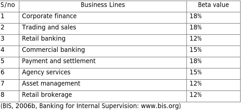
-(Chernobai, A, 2007) because the capital charge is allocated according to a fixed percentage of income currently 15%. The BIA is mostly used by smaller firms with less complex operational functions. Second in line of difficulty is the Standardised Approach (STA). This is similar to the BIA but rather than basing alpha on a single percentage, it sets separate percentages (betas) for each of the eight business lines. Table 2.2 below depicts the eight BCBS business lines with their corresponding values for beta.
TABLE 2.1 THE EIGHT BUSINESS LINES
S/no Business Lines Beta value
1 Corporate finance 18%
2 Trading and sales 18%
3 Retail banking 12%
4 Commercial banking 15%
5 Payment and settlement 18%
6 Agency services 15%
7 Asset management 12%
8 Retail brokerage 12%
(BIS, 2006b, Banking for Internal Supervision: www.bis.org)
The most complex and commonly used approach in measuring operational risk capital charge is the Advanced Measurement Approach which will be explored in broader outlines in the next section.
2.2.2 ADVANCED MEASUREMENT APPROACH
As the name implies, this approach is the most flexible, most advanced and most complex of the three approaches in assessing economic capital. Under
quantitative criteria for the self-assessment
[image:26.595.71.530.342.552.2]27 | U 1 0 4 3 8 5 3 with the administration and regular review of a sound internal operational risk measurement approach (Gregoriou, G, 2009). On the other hand, the quantitative aspect includes the use of both internal and external data, stress testing and scenario analysis, Bayesian methods, business environment and internal control factors. Interestingly, under the AMA approach, a bank has to demonstrate that its operational risk measure is in parity with its internal ratings based approach for credit risk. This implies t
period at 99.9th percentile confidence interval. Jobst (2007) was critical of the practicability of this confidence interval and rather suggested the use of the Extreme Value Theory (EVT) at 99.7% confidence interval in estimating VAR. More so, owing to the flexibility of the AMA, banks are allowed to literally adjust their total operational risk up to 20% of the total operational risk capital charge. Due to the popularity of the AMA, three alternative methods were proposed in 2001: these are the Internal Measurement Approach (IMA), the Scorecard Approach (SCA), and the Loss Distribution Approach (LDA). 2.2.2.1 THE LOSS DISTRIBUTION APPROACHES
A well-known AMA method is the Internal Measurement Approach (IMA) wherein the capital charge is derived by the product of three parameters. These are the gross profit, the probability of event, and the loss given the event. The product of these parameters is then used to calculate the expected loss (EL) for each business line. A second AMA method is the Scorecard Approach (SCA) which is qualitatively skewed approach. Under this approach, banks will have to determine an initial level of operational risk capital based on the BIA or TSA at the business line and subsequently modify the amounts over time on the basis of the scorecards (Chernobai, A, 2007). In other words, the scorecard approach is meant to reduce the frequency and severity of future operational losses by putting in place a proper risk control mechanism for effective risk management. A Scorecard approach is
28 | U 1 0 4 3 8 5 3 Paramount among the AMA methods is the Loss Distribution Approach (LDA) which is most widely used and hence, most popular among risk managers. A
losses are a reflection of its underlying operational risk exposure (Kalkbrener & Aue, 2007). Although operational risk modelling is a recent development in banking, LDA has been used by actuaries to model capital at risk calculation for many years. The LDA is considered the most robust and valid estimate for operational risk exposure (Soprano, A, 2009). Unlike the SCA, this approach uses the exact operational loss frequency and severity distributions to model economic capital. The LDA was suggested by the Basel Committee in 2001 owing to its popularity and success in the actuarial
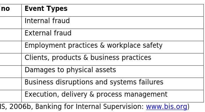
event types besides the business lines (see Table 2.1). This is known as business line/event type matrices. The table below is the seven event type matrix suggested by the BCBS.
TABLE 2.2 THE SEVEN EVENT TYPES
S/no Event Types
1 Internal fraud 2 External fraud
3 Employment practices & workplace safety 4 Clients, products & business practices 5 Damages to physical assets
6 Business disruptions and systems failures 7 Execution, delivery & process management
(BIS, 2006b, Banking for Internal Supervision: www.bis.org)
[image:28.595.84.443.420.616.2]29 | U 1 0 4 3 8 5 3 confidence interval for each business line/event type (BCBS, 2005). The 99.9% confidence interval implies that there is only 0.1% chance that a bank will not have enough capital to cover catastrophic operational losses (DeGroot, M, 2002). Hence, the capital charge is determined by the summation of 56 paired business lines/event types capital charge. From the foregoing, it can be seen that one advantage of the LDA over the IMA is that the former assesses unexpected losses directly while the latter does so via an assumption of the existence of a linear relationship between expected and unexpected losses. Also, unlike in IMA, there is no requirement for risk managers to rescale the expected losses to with a view to determining the unexpected losses. The major shortcoming of the LDA is that it is very difficult to estimate. More so, the use of internal and external operational loss data for the past five years is also a major challenge for banks who have not kept an audit of such historical losses. The use of external data to supplement internal data is advocated by Cope & Willis (2008) who found in a study that a 20 to 30% reduction in predictive error was possible by combining the two sets of data. As stated elsewhere in this thesis, banks are required to estimate the loss frequency and loss severity distributions in order to calculate the capital charge. This process possesses a major challenge for virtually all the banks and will be explored in broader outline below with a particular emphasis on the loss frequency.
2.3 FREQUENCY AND SEVERITY DISTRIBUTIONS
operational losses on the basis of the frequency and severity distributions of each of the BL/ET cell matrix (Kalkbrener & Aue, 2007). While the frequency of event refers to the number of loss event that occur in a given time interval, the severity of event looks at the loss size for each event. The table below illustrates the various types of distributions that can be used to model the frequency and severity of operational losses.
30 | U 1 0 4 3 8 5 3
FREQUENCY DISTRIBUTIONS SEVERITY DISTRIBUTIONS
Poisson Lognormal
Negative Binomial Exponential
Binomial Weibull
Geometric Gamma
Discrete Uniform Beta
Bernoulli Pareto
Hyper Geometric Burr
Logarithmic Normal
Cauchy Rayleigh
In general, loss frequencies can be modelled using a discrete distribution, while loss severity uses a continuous distribution as shown in the table above. The next section will explore the frequency distributions with a particular emphasis on the Poisson and the negative binomial distributions. For details on the severity distributions which model the loss size (see Cruz, G 2002; Soprano, A, 2009; Chernobai, A, 2007). These details are beyond the scope of this thesis and will not be explored further.
2.3.1 FREQUENCY DISTRIBUTIONS
31 | U 1 0 4 3 8 5 3 be likened statistically to discrete random variables. A random variable X is said to have a discrete distribution, if X can take only a finite number of values (DeGroot, M, 2002). The probability of this frequency can be calculated by applying any of the frequency distribution functions in Table 2.3. Each of these discrete probability density functions will be explored in the next section.
2.3.1.1 THE BINOMIAL DISTRIBUTION
Binomial distribution represented by B(n, p) is a discrete distribution that can be applied to model the frequency of operational losses in a given interval of
which has only two outcomes, success and failure, with probabilities p and 1-p, respectively (Dyer, G, 2003). There are four conditions under which Binomial distribution can be applied to yield a good model:
There must be a fixed number of trails (n)
The trials must be independent, i.e. one outcome does not preclude or affect the other outcome
The trials must have only two outcomes (success and failure) The probability of success (p) is constant for each trial
(Attwood, G, 2000)
Hence, the probability of r successes in n trials can be given by:
In the context of operational losses, success (r) could imply, for instance, the event that at least one operational loss has occurred in a day. The number of trials (n) could imply the total number of days in question, e.g. 5 working days in a week in which a loss is equally likely to take place. In other words, the probability that a binomial random variable X takes a value r out of n maximum possible trials, i.e. one will observe losses on r days out of n days. In binomial distribution, the mean (X) = np; while the variance (X) = np (1-p). The binomial may provide a better fit for modelling count data where the variance is less than the mean (Cruz, M, 2002). One major setback in using the binomial distribution to model frequency of operational losses is the
P(X=r) = nCr p
r32 | U 1 0 4 3 8 5 3 assumption of the number of trials (n) in the calculation (Ross, 2002). This is perhaps, why this distribution is not widely used (Klugman et al (2004). More so, when p is small and n is large, the binomial can be approximated by using a Poisson distribution. More so, when n is sufficiently large, binomial can also be approximated by a normal distribution. Further details on binomial distribution can be obtained from Ross (2002), Casella & Berger (2001), Klugman et al (2004), Kingman (1993) and Grandell (1997).
2.3.1.2 THE GEOMETRIC DISTRIBUTION
The geometric discrete probability distribution is used to model the
6). In statistical terminology, it models the number of failures (1-p) that will occur before a success (p). It assumes that each event is independent and that a constant probability of success. The probability density function is given by:
The above function describes the geometric probability that an event will happen at the kth interval of time for the first time with a probability of success p. The mean (X) = 1/p; While the Variance (X) = (1-p)/p2. Like the binomial distribution, the geometric distribution is not a popular choice in modelling frequency of operational losses. This might be because risk managers are not interested in modelling the first time risk occurs but on the frequency of such risk. The most popular distributions used to model risk frequency are the Poisson and the Negative binomial distributions. These two distributions are the bases for this investigation and will be fully explored in broader outlines in separate sections (2.3 and 2.4).
2.4 POISSON DISTRIBUTION
Many experiments consist of observing the occurrence times of random arrivals. Examples include arrivals of customers for service, arrivals of calls at a switchboard, occurrence of floods and other natural, arrival of staff at the office and man-made disasters. Hence, the estimation of the probability of such arrivals becomes necessary in order to study such events. Poisson
P(X=k) = (1-p)
k-1p, k=1, 2,
33 | U 1 0 4 3 8 5 3 distribution can be used to model the number of such arrivals that occur in a fixed period of time. In operational risk, Poisson process can be used to model the frequency of operational losses which is requisite in estimating the regulatory operational value at risk. The Poisson distribution is certainly one of the most popular frequency estimation due to its simplicity of use (Cruz, 2002). Let k be a discrete random variable with a non-negative integer, then k is said to be a Poisson distribution with probability density function given by:
Var (k) = λ; Mean (k) = λ, where k = number of events.
The most attractive and simplistic property of the Poisson distribution is that it assumes a constant mean. Hence, to fit a Poisson distribution to data, one only needs to estimate the mean number of events in a defined time interval. This distribution is particularly used when the mean number of operational losses is somewhat constant over time.
2.4.1 WHY CHOOSE THE POISSON DISTRIBUTION
34 | U 1 0 4 3 8 5 3 more data without structurally changing the analysis. In operational risk, this might involve the addition of a particular business line to the model as in the LDA method of AMA. A good reason for the use of Poisson distribution is the fact that the Mean and Variance is equal. This can provide a quick check on whether a Poisson might be the appropriate distribution for use (Deeks, S, 1999). If the mean and variance of the set of data is not significantly different, this is an indication that a Poisson can be used. Furthermore, another attractive consideration for applying the Poisson distribution is its scalable time-length attribute (Deeks, 1999), i.e. if that the average number of operational losses in a day is 5; then the mean and variance of the corresponding Poisson process are also 5; then it is expected that the number of losses in a 4 day period will be 4 x 5 = 20. As in the case of a truncated data earlier mentioned, this property also makes it very easy for risk managers to adjust the length of time under consideration without structurally changing the database analysis. A further consideration for the use of the Poisson process is the ability to determine its inter-arrival time between events (the length of time between two successive events). The mean of a Poisson is inversely proportional to the mean inter-arrival time. For instance, if in a 10 day interval we expect to witness 7 loss events, then we will expect the mean inter-arrival time to be 10/7 = 1.4 days between events. However, a major setback of the Poisson distribution is its assumption of a constant rate of loss occurrence over time (Soprano, et al, 2000). In reality, the frequency of most operational losses is not constant over time with the mean and variance significantly different. In such a situation, the Negative Binomial distribution may be appropriate. This will be explored in a broad outline in the next section.
2.5 NEGATIVE BINOMIAL DISTRIBUTION
35 | U 1 0 4 3 8 5 3 might let it run until it produces a fixed number of errors and then repair it. This number of failures (n) until a fixed number of successes (r) has a distribution which can be modelled with the Negative Binomial Distribution (NBD). In operational risk terms, the number of failures (n) until a fixed number of successes (r) can imply the number of days (n) that elapsed before a fixed number of operational losses (r) was observed.
The NBD is given by the formula:
Where:
n = Number of events.
r = Number of successful events.
p = Probability of success on a single trial.
2.5.1 WHY CHOOSE THE NEGATIVE BINOMIAL
Earlier applications of the NBD have been used to model animal population (Anscombe, 1949; Kendall, 1948); the number of accidents (Greenwood & Yale, 1920; Arbous & Kerrich, 1951) and in consumer spending patterns (Ehrenberg, 1988). The NBD is probably the most popular distribution in operational risk after the Poisson distribution (Cruz, G, 2002). This is because it has two parameters unlike the Poisson which has one. This availability of two parameters in NBD allows for greater flexibility in the shape of its distribution. This two-parameter property relaxes the assumption of a constant rate of loss occurrence over time assumed by the Poisson. More so, empirical studies conducted by some researchers (Moscadelli, 2004; Rosengren, 2003) have shown that the NBD is a good model for estimating the frequency of operational losses. Unlike in Poisson, the NBD does not assume that the Mean and Variance is equal; rather it assumes that the Variance is greater than the Mean. Hence, to determine whether a set of data is appropriate for the NBD, one can check whether the
P(X = r) =
n-1C
r-1p
r36 | U 1 0 4 3 8 5 3 Variance is greater than the Mean. This assumption further allows for over dispersion in the data (Osgood, 2000). It can be seen from the foregoing that a NBD is a special generalised case of the Poisson distribution in which the intensity rate, λ, is no longer constant but can follow a Gamma distribution with a transformed λ = m, k. Where m = mean, while k is a measure of dispersion of such distribution. This implies that λ has now been split into two parameters to consider the inherent dispersion in the data set. 2.6 EMPIRICAL STUDIES ON POISSON AND NEGATIVE BINOMIAL
It has been noted that the Poisson and the NBD are the most popular distributions of modelling operational risk frequencies and were also recommended by the BCBS. It was also noted that these two distributions differ by their mean and variance. While Poisson assumes equal mean and variance, NBD assumes that the variance is greater than the mean. Hence, choosing between these two distributions require the analyst to compute these two measures of location (mean) and the dispersion (variance) and hence, decide which one to use (DaCosta, L, 2004; Kalkbrener, 2007;
also be used to determine which distribution is most appropriate for the data. This test compares the discrepancies between the observed and the expected frequencies carried out using a test of hypothesis at certain confidence interval.
37 | U 1 0 4 3 8 5 3 better fit than the Poisson distribution (Moscadelli, M, 2004). In a similar vein, De Fontnouvelle et al (2005) examined the data analysed by Moscadelli (2004) but analysed the data on bank by bank basis rather than as a whole. They consider the Poisson and the NBD and concluded that the Poisson provides a better fit than the NBD. This result is also consistent with their earlier study in 2003. In a more recent study, Lewis & Lantsman (2005) examine industry-wide losses due to unauthorised lending over a period 1980 to 2001. Losses below $100,000 for smaller firms and $1,000,000 for larger firms were excluded. They considered the Poisson model and concluded that the mean frequency of loss per year is λ = 2.4 (Lewis & Lantsman, 2005). In a similar vein, Cruz (2002) simulates internal fraud data of a hypothetical commercial bank. He fitted the Poisson model and reported a mean daily frequency of loss of λ = 4.88.
Earlier studies also applied both the Poisson and NBD to model frequencies prior to the advent of operational risk. Sakamoto (1973) carried out a study to determine whether either the Poisson or the NBD better models the frequency of thunderstorm in Nevada, United States. He fitted the data using the Poisson and the NBD and concluded that the NBD is a better model (Sakamoto, C, 1973). In another earlier empirical study (Bortkiewicz, 1898) examined data collected from the Prussian army on the daily number of soldiers kicked to death by horses. He analysed the data using the Poisson
data (Bortkiewicz, 1898). Furthermore, in a more recent study to model the measure of the influence of risk on crime incident counts, Piza, E (2012)
test identified that the NBD is more appropriate for the data. 2.7 SUMMARY OF CHAPTER
38 | U 1 0 4 3 8 5 3 et al 2005 & 2003; Bortkiewicz, 1898) advocated for the use of the Poisson; while some (Moscadelli, 2004; Sakamoto, 1973; Rosengren, 2003; Piza, 2012) advocated for the use of the NBD. Furthermore, some studies (DaCosta, 2004; Kalkbrener, 2007; Osgood, 2000) advocated the use of the Poisson when the mean is somewhat equal the variance; the NBD when the variance is greater than the mean; and the Binomial distribution when the variance is less than the mean. More so, some authors (Cruz, 2002; Chernobai, 2007; Klugman, 2004) advocated the use of ratio tests, especially
by comparing observed and expected frequencies. In the light of the above, it can be deduced from the literature that the most popular distributions are
there is no clear choice between the Poisson and the NBD because the choice of severity in calculating the operational value at risk outweigh that of the frequency. Hence, this answers my research questions:
1. Is there a significant difference from the results obtained in the use the Poisson and Negative binomial distributions in modelling the frequency of operational risk losses?
2. Under what conditions should we adopt one for the other?
CHAPTER THREE
3. RESEARCH METHODOLOGY
39 | U 1 0 4 3 8 5 3 description should be detailed enough to allow any interested party to be able to replicate the study. This detailed description normally includes: methods, procedures, sampling, research questions, data source, data analysis, instruments, ethical issues and limitation of study.
This study investigated the two major methods of modelling the frequency of operational losses under the BCBS Accord of 1998 known as Basel II Capital Accord. It compared the Poisson method of modelling the frequency of losses to that of the NBD. The frequency of operational losses was investigated using a cross section of secondary data published by the Banking for International Settlements (BIS) collected in the 2002 Loss Data Collection Exercise for Operational Risk.
3.1 POPULATION AND SAMPLING
Sampling is the method used in selecting a subset of the population for study. There are various types of sampling methods: simple random, quota, census, systematic, stratified, cluster, convenience and multi-stage sampling. On the other hand, Sample is the data selected from a population for study with a view to making generalisation about the population from which it was drawn. Whereas, population refers to the total number of objects or people that a researcher is interested in studying. For the purpose of making comparison and ease of data collections, Basel II grouped the 89 banks from 19 countries that participated into five regions. Hence, the population of this study comprises all financial institutions in the four Basel II regions of Europe, Australasia, North and South America, and Asia. In order to eliminate sample error (errors as a result of sampling), as well as increase internal validity, the sample of my study consisted of the entire 89 banks (census) from 19 countries worldwide that participated in the 2002 LDCE. Census study was considered most appropriate since secondary data would be used. Census would also ensure that any interpretation is a true representation of the population.
3.2 VALIDITY AND RELIABILITY OF INSTRUMENTS
40 | U 1 0 4 3 8 5 3 Validity can be external or internal. External validity refers to generalising
extent to which the stated interpretation of the result is
2000). From these definitions, internal validity merely refers to the validity of the sample and does not aim to generalise the result. The term reliability, in lar
words, this refers to the consistency in measurement. The validity and reliability of this study was ensured by using well known theoretical frameworks for modelling count events. These are known as the Poisson distribution and the Negative Binomial distribution; for details of the Poisson and the NBD see Cruz, 2002. More so, since the LDCE was conducted by the BCBS (an international body made up of governors of prominent Central Banks worldwide), the published 2002 LDCE data was deemed to be valid and reliable.
3.3 DATA COLLECTION
The frequency of operational loss events will be investigated using a cross section of secondary data published by the Banking for International Settlements (BIS) resulting from the 2002 Loss Data Collection Exercise (LDCE) for Operational Risk. A total of 89 banks from 19 countries were
occurred in the year 2001. They were also required to categorise the data into the standardised 8 business lines and 7 event types. The frequencies of loss events were also aggregated quarterly, weekly and daily by all the banks as a requirement. Overall, the 2002 LDCE reported 47,269 individual loss
41 | U 1 0 4 3 8 5 3 3.4 DATA ANALYSIS
This study analysed the distribution of daily frequencies of operational loss data collected by the Risk Management Group (RMG) of the BCBS in 2002 as mentioned in the preceding section above. The data were classified into eight business lines (Table 2.1) and seven event types (Table 2.2) pooled together across all banks not only to protect the identity of the participating banks, but also to compare the operational riskiness of each BL/ET. The Poisson and the NBD models were fitted to the daily number of loss events on 3 of the 8 business lines with a view to drawing conclusions on which model provides a better fit. The models were at first fitted on the overall data aggregated daily; it then went further to fit the models these business lines: Corporate Finance, Trading and Sales, and Retail Banking. The statistical software used to fit the data the XLSTAT 2013 and the EASYFIT 5.5 Professional edition. The XLSTAT 2013 was used mainly to carry out the Chi Square goodness of fit test while, the EASYFIT 5.5 was used to draw the graphs and charts as well as calculate the parameters of the data.
3.4.1 GOODNESS OF FIT TESTS
42 | U 1 0 4 3 8 5 3 3.4.1.1.
While the Likelihood Ratio (LR) test is the most common formal test applied
Goodness of Fit test on the other hand, is the most common test applied to discrete probability distributions such as the NBD, Binomial and the Poisson (Chernobai, 2007). The PCS test checks whether the data sample follows a hypothetical distribution. In this case, whether the observed frequencies fit the Poisson or the NBD frequencies. Hence, the PCS test was considered most appropriate for this study.
3.4.1.2 HYPOTHESES TESTING
In order to determine whether the correct model has been used in this study, the following statistical hypotheses were tested at 5% significant value using n-p-1 degree of freedom. The test that was used is the widely used
1. H0 (Null hypothesis): the frequency of operational losses in banks follows the Poisson distribution.
2. H1 (Alternative hypothesis): the frequency of operational losses in banks does not follow the Poisson distribution.
3. H0 (Null hypothesis): the frequency of operational losses in banks follows the Negative Binomial distribution.
4. H1 (Alternative hypothesis): the frequency of operational losses in banks does not follow the Negative Binomial distribution
Thus, if the value of Chi-square at n-1 degree of freedom is less than the critical value, then the Null hypothesis will be rejected and the Alternative hypothesis will be accepted. On the other hand, if the value of the Chi square is greater than the critical value, the Null hypothesis will be accepted and the
43 | U 1 0 4 3 8 5 3 distribution is used for a particular set of business lines. The decision to test at 5% significance, i.e. 95% confidence interval is to reduce the likelihood of Type 1 Error (falsely rejecting H0 when in fact, H0 is true). For the Chi Square critical value table that was used, please see Appendix B.
3.5 ETHICAL CONSIDERATION
To ensure that ethical standards were met, the need to protect the identities of individual banks, as well as their respective losses became paramount in this study. To ensure anonymity, the names and addresses of participating banks were not published by the BCBS, as well as the amount of individual losses. Rather, the losses were pooled together and categorised into the standard 8 BLs and 7 ETs. Furthermore, the operational loss data collected by the Risk Management Group (RMG) of the Banking for International Supervision in the 2002 are available in the public domain at www.bis.org. No special permission needed to be sought before the use of these data. More so, ethical approval was sought from the University prior to the commencement of this thesis in the form a written proposal (Appendix C) 3.6 LIMITATION OF STUDY
44 | U 1 0 4 3 8 5 3 CHAPTER FOUR
4. DATA ANALYSIS
45 | U 1 0 4 3 8 5 3 making comparisons of the results obtained from fitting the Poisson and the NBD to the observed frequency in order to answer my research questions:
1. Is there a significant difference in the use the Poisson or Negative binomial distributions in modelling the frequency of operational risk losses?
2. Under what conditions should we adopt one for the other? 4.1 GROUPED FREQUENCY OF LOSS EVENTS
The number of individual loss events that occurred in the year 2001 as reported by the 89 banks that participated in the 2002 LDCE of the BCBS (see Sections 3.3 & 3.4). The overall distribution of this data is the subject of analysis and discussion in this section. The table below depicts this information.
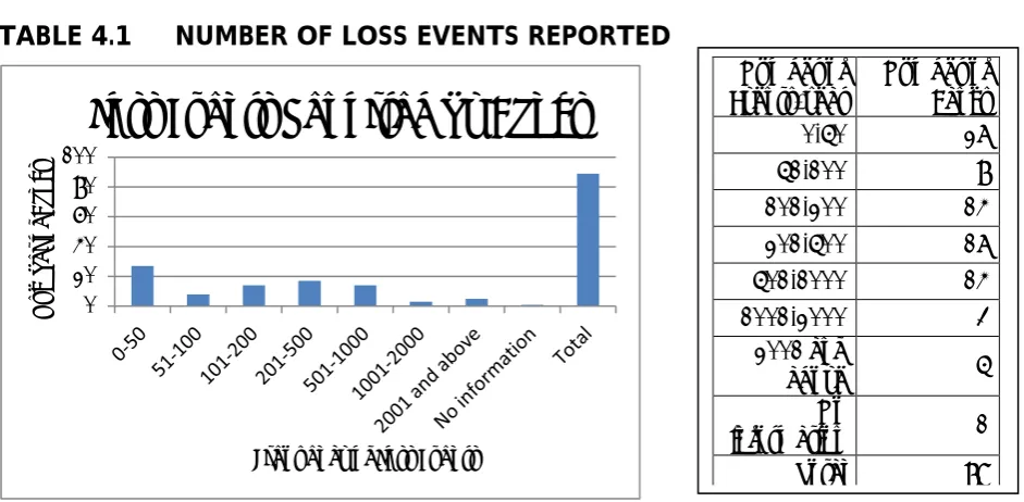
[image:45.595.73.544.375.606.2]FIGURE 4.1 NUMBER OF LOSS EVENTS REPORTED
TABLE 4.1 NUMBER OF LOSS EVENTS REPORTED
The figure above illustrates that the range of individual loss events reported by these banks was quite large, with values ranging from only 1 event to as large as 2,000 events. Over half of the banks (55%) reported 200 or less number of events, and the majority of these (55%) reported fewer than 50 events. On the other hand, 8 banks reported over 1,000 individual loss events, and 5 reported more than 2,000 loss events. Since the modal
0 20 40 60 80 100 N u m b e r o f B an ks
Frequency of Loss Events
Loss Events Reported by Banks
Number of Events/year
Number of Banks
0-50 27
51-100 8
101-200 14
201-500 17
501-1000 14
1001-2000 3
2001 and
above 5
No
information 1
46 | U 1 0 4 3 8 5 3 number of loss events per year is 0-50, it can be concluded that the average number of loss events per year encountered by banks is up to 50.
4.1.1 FREQUENCY OF LOSSES BY BUSINESS LINE/ EVENT TYPE
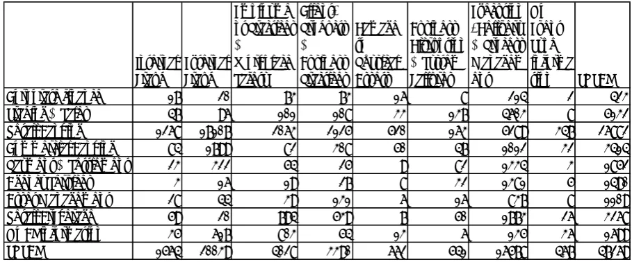
The basic features of the individual loss data submitted by all the 89 participating banks are the subject of analysis and discussion in this section. Hence, the table below illustrates the total number of individual loss events reported by each of the 89 banks in combinations of the 8 BL and 7 ET amounting to 56 separate cells. The data was classified according to BL/ET and pooled together across all the 89 banks.
TABLE 4.2 FREQUENCY OF LOSS EVENTS PER BL/ET
For the purpose of in depth analysis, the above table with values converted to percentages is shown below.
TABLE 4.3 FREQUENCY (PERCENTAGE) OF LOSS EVENTS PER BL/ET Internal Fraud External Fraud Employme nt Practices & Workplace Safety Client, Products & Business Practices Damage to Physical Assets Business Disruption & System Failures Execution , Delivery & Process Managem ent No Event Type informa tion TOTAL
Corporate finance 17 20 73 73 16 8 214 2 423
Trading & Sales 47 96 101 108 33 137 4603 8 5132
Retail Banking 1268 17107 2063 2125 520 163 5289 347 26882
Commercial Banking 84 1799 82 308 50 47 1012 32 3414
Payment & Settlement 23 322 54 25 9 82 1334 3 1852
Agency Services 3 16 19 27 8 32 1381 5 1490
Asset Management 28 44 39 131 6 16 837 8 1109
Retail Brokerage 59 20 794 539 7 50 1773 26 3268
No BL information 35 617 803 54 13 6 135 36 1699
[image:46.595.71.526.306.495.2]47 | U 1 0 4 3 8 5 3 From the tables above, a total of 47,269 individual loss events categorised according to their corresponding BL/ET cells. It can be noticed that the events are not evenly spread across BL/ET. In particular, the data were clustered into half of the 8 BL, with the highest concentration in Retail Banking. This BL accounted for 61% of the total number of loss events. Hence, it can be drawn that Retail Banking accounts for more than half the number of operational loss events. This finding is consistent with (Cruz, 2002; Chernobai, 2007; Moscadelli, 2004). Trading and Sales accounted up to 11%, while commercial Banking and Retail Brokerage, each accounted for 7%. Thus, these 4 BL accounted for 86% of all individual loss events. On the other extreme, Corporate Finance is the fewest with just below 1%. A similar pattern of clustering is apparent in the ET category with 42% categorised as External Fraud; 35% as Execution, Delivery and Process Management; Employment Practices and Workplace Safety 9%; and Client Product and Business Practices accounting for 7%. These four categories accounted for 93% of individual loss events. On the individual BL/ET cell category, a clustering can also be found in the Retail Banking/External Fraud cell with 36% of loss events reported. It can be drawn from the data that the number of operational loss events due to fraud in retail banking accounts for up to 40% of losses.
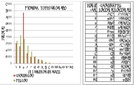
48 | U 1 0 4 3 8 5 3 4.2 DISTRIBUTION OF DAILY FREQUENCY OF LOSS EVENTS
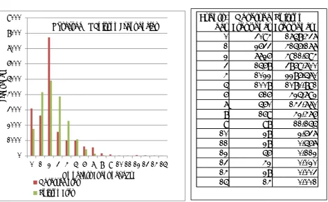
In this section, the 47,269 individual loss events reported by the 89 banks in the 2002 LDCE but aggregated daily will be explored in broader details. The number of loss events in this case has been grouped on a daily basis, i.e. total number of loss events that occurred per day. Table 4.4 is an illustration of these daily loss events.
FIGURE 4.2 FREQUENCY OF LOSS EVENTS- AGGREGATED DAILY
49 | U 1 0 4 3 8 5 3 In the above table, notice that the total observed frequency is 18,690. The total number of observations of 47,269 was obtained by multiplying the number of events/day (column one) with the corresponding observed frequency (column two) which were summed and added to the number of zero events (3,094). Analysing the figure above, It can be drawn that the average number of operational loss events is two per day accounting for 41% of the total loss events. This modal number of 2 loss events per day is consistent with Cruz (2002) who examined the frequency of 3,338 operational loss events obtained from a major British retail bank from 1992 to 1996; he obtained a mode of 2 loss events per day (525/1311) which also accounted for 40% of number of loss events (Cruz, M, 2002, p95). This is followed by no loss events per day with 17%; then 3 loss events per day at 14% which decreases in value as the number of loss increases. A fifteen loss events per day is the smallest, as one will expect, with less than 1%. By observation, it can be seen from the figure that the distribution appears to be positively skewed as the tail of the distribution is longer on the right. It can be concluded that the frequency distribution of operational loss events is
0 1000 2000 3000 4000 5000 6000 7000 8000 9000
0 1 2 3 4 5 6 7 8 9 10 11 12 13 14 15
Ob ser ve d Fr e q u e n cy
No of Loss Events per day
FREQUENCY OF DAILY LOSS EVENTS IN THE YEAR No of
events/day
Observed frequency
0 3094 (16.5%)
1 2633 (14.0%)
2 7726 (41.3%)
3 1568 (8.3%)
4 1022 (5.4%)
5 1008 (5.3%)
6 616 (3.3%)
7 560 (3.0%)
8 169 (0.9%)
9 98 (0.5%)
10 28 (0.015%)
11 28 (0.015%)
12 56 (0.30%)
13 42 (0.22%)
14 28 (0.15%)
15 14 (0.01%)
50 | U 1 0 4 3 8 5 3 positively skewed. An exploration of the statistical parameters of this distribution will be carried out in the next section to further investigate its characteristics in broader details.
4.2.1 DESCRIPTIVE STATISTICS
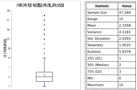
[image:50.595.75.522.277.569.2]A summary of the descriptive statistics and box plot for the frequency of the daily loss events in the year as shown in Table 4.4 above is shown below: FIGURE 4.3 BOX PLOT OF FREQUENCY OF LOSS EVENTS
TABLE 4.5 STATISTICS OF FREQUENCY OF LOSS EVENTS
The data has a skewed parameter of 1.9525 which confirms that it is positively skewed. Recall that a skew parameter of zero is a symmetrical distribution; and less than zero is a negatively skewed distribution. The above box plot further confirms this assertion. More so, since the mean (2.3358) is more than the median (2), this further confirms positive skewness. From the box plot above, the outliers (extreme values) are
number of e
here with the operational number of loss events which could exceed 15 loss
0 2 4 6 8 10 12 14 16 No of ev e nt s/d ay
Frequency of Daily Event in the Year) Statistic Value
Sample Size 47,269
Range 15
Mean 2.3358
Variance 4.1181
Std. Deviation 2.0293
Skewness 1.9525
Kurtosis 5.9379
25% (Q1) 1
50% (Median) 2
75% (Q3) 3
Min 0
51 | U 1 0 4 3 8 5 3 events per day in very large multinational banks, I will not be considering the statistical concept of excluding outliers in this calculation. However, it can be concluded from the above figure that any number of loss events exceeding 6
number of loss events per day can be considered normal if it is between 0 and 6.
From Table 4.5, the range is 15 and the standard deviation is 2, which shows high spread and variability in the number of loss events reported per day among the banks. The Lower Quartile (Q1-the 25% position of the data) is 1 and the Upper Quartile (Q3- the 75% position of the data) is 3. Hence, the IQR = Q3 Q1 = 2. The IQR measures the middle 50% of the data in a bid to rid the data of any extreme values from both directions. Another important parameter for consideration is the kurtosis. This measures the spread of the values around the mean, i.e. the peakedness of the data. A high kurtosis implies a high peak in the centre of the data. A population with a high kurtosis is called leptokurtic. As a general rule of thumb, if the kurtosis value of a distribution is above 3, such is referred to as leptokurtic and cannot be represented by a normal distribution (Cruz, 2002, p40-43). Since my kurtosis value is 5.9379 from Table 4.5, It is suffice to generally conclude that the daily distribution of the number of loss events has a high kurtosis and hence, leptokurtic.
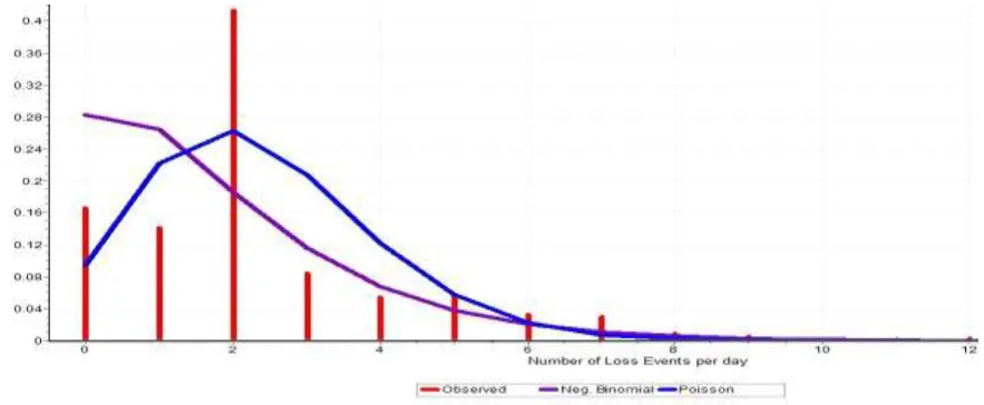
Furthermore, from Table 4.5 the mean is 2.3358 and the variance is 4.11. Since the variance is significantly greater than the mean, it is tempting for one to conclude that the NBD will fit the distribution better than the Poisson (see Section 2.6). However, such conclusion may be inconclusive without first fitting the observed frequency to the theoretical frequency on both the Poisson and the NBD. This will be the basis of the next two sections 4.22 and 4.23.
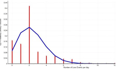
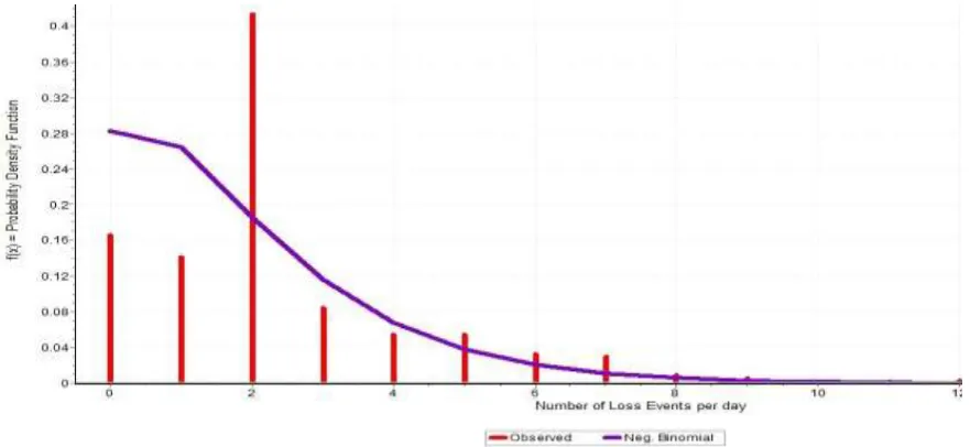
4.2.2 TESTING THE POISSON FIT TO THE DATA
The figure and table below show the observed frequency as it compares with that of Poisson frequency.