Stratus: Load Balancing the Cloud for Carbon Emissions Control

Stratus: Load Balancing the Cloud for Carbon

Emissions Control

Joseph Doyle, Robert Shorten, and Donal O’Mahony

Abstract—Large public cloud infrastructure can utilise power which is generated by a multiplicity of power plants. The cost of electricity will vary among the power plants and each will emit different amounts of carbon for a given amount of energy generated. This infrastructure services traffic that can come from anywhere on the planet. It is desirable, for latency purposes, to route the traffic to the data centre that is closest in terms of geographical distance, costs the least to power and emits the smallest amount of carbon for a given request. It is not always possible to achieve all of these goals so we model both the networking and computational components of the infrastructure as a graph and propose the Stratus system which utilises Voronoi partitions to determine which data centre requests should be routed to based on the relative priorities of the cloud operator.

Index Terms—Voronoi Partitions, Cloud Computing, Load Balancing, Carbon Emissions

F

1

I

A variety of new services are being offered under the cloud computing paradigm. This service model involves a cloud based service provider (CBSP) pro-viding a large pool of computational and network resources which are allocated on demand to the cloud users from the pool. Cloud users in turn can use these resources to provide services for users. The pool of resources can comprise of several data centres (DCs) at different geographical locations. There are many potential benefits to a global distribution of servers if load balancing is used correctly. Reduced latency and increased data transmission rates can be achieved by assigning clients to servers which are closer in terms of link distance. For some applications such as conference Voice-over-IP (VoIP) software and interactive online games low latency is critical in order to provide a satisfactory Quality of Service (QoS). In addition, there have been proposals to consider electricity price when load balancing [1], [2], [3] to reduce operational costs. By assigning more load to a DC which is utilising relatively cheap electricity operational costs can be lowered. This load balanc-ing can be achieved with protocol-level mechanisms which are in use today such as dynamically generated DNS responses, HTTP redirection and the forwarding of HTTP requests. All of these have been evaluated thoroughly [4], [5], [6].

Recently the carbon emissions associated with pow-ering DCs have become important. Greenpeace report [7] the carbon emissions of selected DCs and the per-centage of their electricity generated by power plants that use fuels which emit a relatively large amount

• J.Doyle and D.O’Mahony are with the CTVR research group in Trinity College Dublin, Ireland.

• R. Shorten is with IBM Research.

of carbon. The carbon intensity of a power plant is the carbon emitted for a given amount of energy generated. The carbon intensity of power plants using particular fuels is detailed in [8], [9]. Currently there is little financial motivation to use green or clean energy but increasing regulation of carbon emissions and schemes like the European Union Emissions Trading Scheme (EU ETS) [10] mean that in the future it is probable that the right to emit carbon into the atmo-sphere will be traded as a commodity. In addition, recent work [11] suggests that on-site power genera-tion can reduce carbon emissions and electricity cost by reducing the peak draw of a data centre from an electricity supplier.

There have been some proposals to use locally generated clean energy [12] or employ load balancing based upon the carbon intensity of the electricity sup-plier [13]. These proposals, however, do not consider the carbon emitted as a results of packets travelling across the network from the client to the server. While the energy consumed by the networking equipment as part of the cloud computing has been analysed [14], additional analysis is required to examine the total carbon emission caused by a cloud computing system. In addition, other proposals for minimising carbon emissions use weather data as a metric for load balancing. While this is a useful metric for in-house generated electricity it can be inaccurate when elec-tricity is obtained from an external supplier as other factors affect their carbon intensity. This is discussed in greater detail in Section 5.2. Carbon emissions are seldom the sole concern of cloud operators and other factors must be considered. The electricity cost can vary considerably between different geographical re-gions and this fact can be exploited by cloud operators to lower the operational cost.

as certain schemes such as “free air cooling” require less energy and hence emit less carbon. Finally cloud operators are usually bound by service level agree-ment (SLA) and therefore must maintain a minimum QoS for service users.

It is not always possible to achieve the best case sce-nario for all of these factors as they sometimes conflict, so we formulate a graph-based approach which we call Stratus that can be used examine and control the operation of the cloud. Stratus uses Voronoi partitions which are a graph-based approach which have been used to solve similar problems in other areas such as robotics [15]. In this paper we use this approach to attempt to control the various factors which affect the operation of the cloud. This paper makes the following contributions:

• The development of a model which details the carbon emissions, electricity cost and time re-quired for the computational and networking aspects of a service request.

• A distributed algorithm which minimises the combination of average request time, electricity cost and carbon emissions is described.

• Data for the carbon intensity and electricity price of various geographical regions and a represen-tative set of round trip time between various geographical regions is presented.

• We evaluate the performance of our distributed algorithm using the data obtained for various scenarios.

2

R

W

There have been a number of proposals which con-sider the cost of electricity when determining which data centre should service requests. Qureshiet al.[1] proposed a distance-constrained energy price opti-miser and presented data on energy price fluctuations and simulations illustrating the potential economic gain. Stanojevicet al.[2] detail a distributed consensus algorithm which equalises the change in the cost of energy. This is equivalent to minimising the cost of energy while maintaining QoS levels. Rao et al. [16] formulate the electricity cost of a cloud as a flow network and attempt to find the minimum cost of sending a certain amount of flow through this network. Raoet al.[17] also propose a control system which uses load balancing and server power control capabilities to minimize energy cost. Wanget al. [18] propose using a corrected marginal cost algorithm to minimize electricity cost. Mathew et al. [19] propose an algorithm which controls the number of servers online in the cloud to reduce energy consumption. It also maintains enough servers at each data center to handle current requests as well spare capacity to han-dle spikes in traffic. Liuet al. [3] propose distributed algorithms which minimize the sum of an energy cost and a delay cost using optimization techniques such

as gradient projection to minimise the overall cost of operating the data centre. In addition, they expand their formulation to consider minimizing the sum of the social impact cost and delay cost. They define the social impact cost as a metric for environmental impact of the data centre. By examining the avail-ability of renewable energy and directing load to the appropriate data centres they attempt to reduce the environmental impact of the data centre.

In addition, there has been some analysis of the electricity consumption of the cloud computing paradigm. Baliga et al. [14] analyse the power con-sumption of all the elements of this for a variety of service scenarios. Mahdevan et al. [20] examine the power consumption of network switches and consider techniques for improving the power efficiency of net-work switches by disabling ports and using lower data rates where possible.

There have also been some proposals which con-sider carbon emissions when determining where to direct service requests. Liuet al.[12] expand the model proposed in [3] to subtract locally generated clean energy from the energy cost calculation to allow data centres which have clean energy generation facilities to service more load. Doyle et al. [13] describe an algorithm that minimizes a cost function containing the carbon intensity of the electricity supplier of the data centre and average job time. Moghaddam et al. [21] attempt to use a genetic algorithm-based method with virtual machine migration to lower the carbon footprint of the cloud. Gao et al. [22] use a flow optimization based framework to control the three way trade-off between average job time, electricity cost and carbon emissions. This system, however, is only evaluated using yearly average carbon intensity values. While the system could be applied to the instantaneous carbon intensity value of an electricity supplier, the evaluation only considers the yearly average which can differ significantly from the instan-taneous value.

Some of these proposals use various mathematical techniques to achieve their goals. In this work we propose the use of Voronoi partitions which are used in a number of areas. Aurenhammer details a number of applications in [23]. Durhamet al.[15] use Voronoi partitions to divide an environment so that a group of robots can provide coverage.

respond to incremental change is required.

3

P

F

In this section we formulate the problem. To do this we need some background notation. Namely we need to say what a graph is; what a Voronoi partition is; and how we use these ideas in the context of cloud computing.

3.1 Graph

A graph consists of a finite set of nodes and edges. Each edge is incident with two nodes. A path is an ordered sequence of points such that any consecutive pair of points is linked by an edge in the graph. In an undirected graph there is no direction associated with the edges. Hence, a path can be constructed with any edge in the graph. A weighted graph associates a label with each edge. Nodes are connected if a path exists between them.

3.2 Voronoi Partitions

Voronoi partitions are the decomposition of a set of points into subsets. These subsets are centered around points known as sites, generators or seeds. Each point in the set is added to a subset consisting of a site and all other points associated with this site. An abstract notion of distance between a point and the sites is used to determine which subset a point is associated with. A point is assigned to a subset if the distance to site is less than or equal to the distance to the other sites. For an example of Voronoi partitions used in applications (robotics) see [15]. We shall now use these partitions to solve routing problem associated with load balancing in the cloud.

3.3 Voronoi Partitions of the Cloud

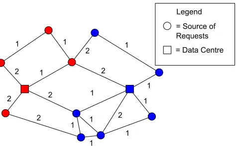
In our work the set of points consist of sources of requests for cloud services and data centres which service these. Voronoi partitions are then used to determine where requests are serviced. A Voronoi cell represents which sources of requests a data centre is servicing at a given time. An example of a group of sources of requests which have been partitioned between two data centres can be seen in Figure 1. In this figure each source of requests has a path to both data centres. The partition that the source of requests is a part of depends on the paths to the two data centres. The partitions are made up of sources of requests which have paths available to them with lower distances than the paths available to the other data centre.

Legend

1

1 2 1

2

2 2

2

2 1

1

2

1 1

1 1

1

1

= Source of Requests = Data Centre

Fig. 1. Example of how sources of requests are

partitioned between two data centres. Colour indicates that the node is part of a particular partition.

3.4 Problem Statement

Let |J| be a set of J geographically concentrated sources of requests and|N|be a set ofN data centres. Let |Q| be a finite set of points that represent either sources of requests or data centres. These points are connected by E edges in an undirected weighted graph G = (|Q|,|E|,|w|). The weights are calculated as functions of the time required to service a fraction of the requestTi, the carbon emissions associated with

servicing the fractionGi and the electricity costEi if

any associated with servicing the request along the edge.

wi=f(Ti, Gi, Ei) =Ti+R1(Gi) +R2(Ei) ∀i∈ |w|

where R1, R2 are the relative price functions which

are used to specify the relative importance of the factors. WhileEiandGiare related, the rates at which

they increase may vary significantly depending on the specifics of the cloud and hence, both must be included in the problem formation to ensure the cloud operator can operate the cloud as desired. It should be noted that the weights of the graph represent the networking and computational aspects of servicing a request.

The set|Q|is partitioned intoN subsets represent-ing the regions serviced by each data centre. This results in a collection P = {Pi}Ni=1 of N subsets of

|Q|such that: 1) SN

i=1Pi=Q

2) Pi∩Pj=∅ if i6=j

3) Pi6=∅ ∀i∈ {1, . . . , N}

4) Pi is connected for all i∈ {1, . . . , N}

Two subgraphsPi and Pj are connected if there are

two verticesqi, qj belonging, respectively, to Pi and

Pj such that(qi, qj)∈ |E|.

We can use Voronoi partitions to establish a collec-tion of subsets which minimizes the combinacollec-tion of carbon emissions, electricity cost and average request time. In this case the Voronoi partitionPi associated

1 U :=Pi(t)∪Pj(t)

2 forx∈U

3 Wi:={x∈U :d(x, i)≤d(x, j)}

Wj:={x∈U :d(x, i)> d(x, j)}

4 endfor

5 Pi(t+ 1) :=Wi

Pj(t+ 1) :=Wj

Fig. 2. Pseudocode for pairwise partitioning rule

0 100 200 300 400 500 600

08/01 02/02 27/02 24/03 18/04 13/05

Peak Day-Ah

ead Elect

ricity Price ($/MWhr)

Date

Virginia Ireland California

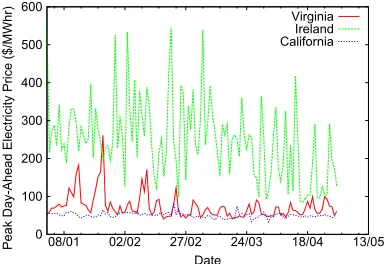
Fig. 3. Peak Daily price of electricity for suppliers in the regions of the three data centres studied.

points whose distance to data centrei is less than or equal to the distance to another data centre j ∈ |N|. We assume that the data centres have sufficient com-putational capacity so that there is no constraint on the size of Pi. In order to compute this we need

to define how the distance between two points is calculated. A standard notion of distance between two pointsd(i, j)in a weighted graph is the lowest weight of a path between the two points (i, j). The weight of a path is the sum of the weights of the edges in the path. The goal of using the Voronoi partitions in this scenario is to minimize the distance between the sources of requests and the data centres. This can be defined as:

min

N

X

i=1 X

j∈Pi d(i, j)

Note if a source is equidistant to more than one data centre the point is assigned to the Voronoi partition that has the least members to attempt to balance the load on the data centres.

A pairwise partitioning rule can be used to achieve this goal.

4

P

P

R

At timetdata centreiand data centrejcommunicate by exchanging the partitions Pi and Pj so that each

data centre can examine all the regions associated with the two data centres to determine if there is a bet-ter route available between a data centre and a region. We assume without a loss of generality that i < j. Each data centre then performs the actions depicted in

0 50 100 150 200 250 300

21/01 22/01 23/01 24/01 25/01 26/01 27/01 28/01

Day-Ahe

ad Electricity P

rice ($/MWhr)

Date

Virginia Ireland California

Fig. 4. Price of electricity for suppliers in the regions of the three data centres studied.

the pseudocode in Figure 2. The paths between each region and the two data centres are examined. If the path between the data centreiand a region is smaller than the path between the region and the data centre j then the region is added to a temporary partition associated with data centre i. Otherwise it is added to a temporary partition associated with data centre j. The partitions of the two regions are then updated with the appropriate temporary partition. In order to generate the initial partitions the distance between each node in the graph and all the data centres is calculated. The nodes are then added to the partition which yields the minimal distance between the nodes and the data centre.

5

C

A

In this section we examine the variation in the costs that exist between data centres.

5.1 Electricity Cost

0 100 200 300 400 500 600 700

08/01 02/02 27/02 24/03 18/04 13/05

Carbon Intensity (g/kW

hr)

Date

Fig. 5. Daily peak carbon intensity of electricity sup-plier in the region of the Ireland data centre studied.

these as they supply electricity in the region the data centres are located. Ireland uses a single market for electricity known as SEMO and only a single price for wholesale electricity is available. The peak daily day-ahead electricity price for these suppliers from January 2011 through April 2011 is depicted in Figure 3.

It is interesting to note that the maximum price can approach $550/MWh and that the peak price for the electricity is nearly always greatest in the Ireland region. This would suggest that little traffic would be routed to the Ireland data centre if a load balanc-ing scheme design to minimise electricity prices was utilised. If, however, we examine the hourly variation of electricity prices we can see that this is not the case. The day-ahead electricity price for the electricity suppliers from the22nd January 2011 through the29th January 2011 is depicted in Figure 4. From this we can see that peaks in electricity price in the Ireland region tend to be very sharp and that at non-peak times the variation in price between geographical regions is much smaller.

5.2 Carbon Emissions

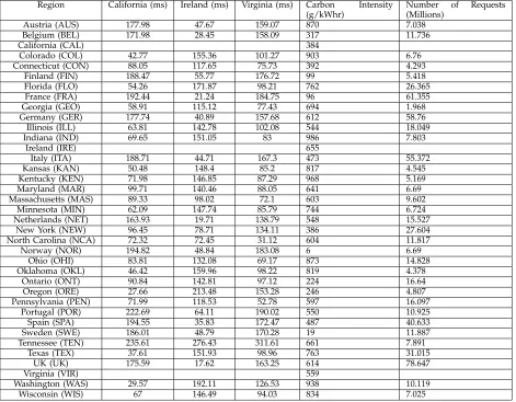
An analysis of the carbon intensity of electricity sup-pliers in various geographical regions is useful when attempting to minimise the environmental impact of a cloud. To illustrate this we examine the carbon emitted by a service which has users in a number of different geographical regions utilising the EC2 infrastructure. The carbon intensity data for the data centres and sources of requests were obtained from [28] and can be seen in Table 1. The data for states in the United States were in agreement with data from [29]. The carbon intensity of an electricity supplier is calculated using the weighted average (where the power generated by the power plant is the weight used) of the carbon intensity of the power plants operated by the electricity supplier. The demand for electricity changes over the course of a day and electricity suppliers turn power plants on and off to

0 100 200 300 400 500 600 700

21/01 22/01 23/01 24/01 25/01 26/01 27/01 28/01 29/010 200 400 600 800

Carbon Intensity (g/kW

hr)

Wind Power Generated

(MW)

Date

Carbon Intensity Wind Power Generated

Fig. 6. Carbon intensity and generated wind power of electricity supplier in the region of the Ireland data centre studied.

react to the changes in the demand. A consequence of this is that the carbon intensity of an electricity supplier varies over time. It would be possible to estimate the realtime carbon intensity by examining the weighted average of the carbon intensity for all the power plants that are operating but some elec-tricity suppliers provide a realtime carbon intensity value directly. To the author’s knowledge, the realtime carbon intensity of all the geographical regions in Table 1 is not available. It is, however, available for the Ireland region. Figure 5 depicts the daily peak carbon intensity of the electricity supplier in Ireland from January through April 2011. This data was ob-tained from the Ireland Transmission System Operator Eirgrid [30]. We can see that there is a large variation with time. This suggests that the data can be exploited to minimise the environmental impact of the cloud. Figure 6 depicts the carbon intensity of the SEMO suppliers from the 22nd _{January 2011 through the} 29th _{January 2011. The interval between data points} is fifteen minutes. From Figure 6 we can see that the carbon intensity is not as volatile as the electricity market price but varies enough to allow the cloud operator to utilise the realtime data to minimise the environmental impact.

plants (e.g. coal) take a long time to turn on or off. The result of this is that they are very rarely turned off and if there is insufficient system demand solar and wind power is wasted.

The second reason that the use of weather data can be an inaccurate metric is that even if there is sufficient demand and solar and wind power is utilised the changes in the operation of other power plants can affect the carbon intensity. As a result there is not a direct correlation between availability of wind and solar power and carbon emissions. For example if a pumped storage plant is turned on and the wind speed drops carbon intensity may still go down. The reason for this is that the reduction in carbon emissions caused by the use of the pumped storage plant may be greater than the increase in carbon emissions caused by other power plants supplying the electricity which is no longer supplied by the wind turbines. If we examine Figure 6 we can see an example of this. There is some correlation between the wind power generated and carbon intensity but it not direct. Sometimes when the wind power generated increases the carbon intensity also increases. It should be noted that the Irish SEMO market does not use significant amounts of solar power so this is not a factor in the analysis.

5.3 Cooling Cost

Cooling costs for a data centre are dependent on its design and the local climate in addition to the load placed upon it. If a data centre uses aisle containment [31] it can significantly reduce the cost of cooling the data centre. Aisle containment is the separation of the inlets and outlets of servers with a barrier such as PVC curtains or Plexiglas [32] in order to prevent air migration which adversely affects cooling costs.

In addition “free air cooling” can be used. This is the use of air economizers to draw in cold air from the environment into the data centre when the climate conditions are suitable, thereby preventing the use of computer room air conditioner (CRAC) chiller units and lowering the cooling costs [33]. Water cooling [34], [35] can also be used but it is rarely used in data centres at present.

In order to examine how this cost varies with demand we constructed two models of data centres in the computational fluid dynamics (CFD) simulation software Flovent [36]. These represent typical data centres which have been examined in previous re-search [37], [38]. One data centre used cold aisle con-tainment and the other does not. Apart from this the data centres were of similar construction. Each data centre has dimensions11.7m×8.5m×3.1m with a0.6m raised floor plenum that supplies cool air through perforated floor tiles. There are four rows of servers with seven 40U racks in each case, resulting in a total of 1120 servers. The servers simulated were based on

0 1 2 3 4 5 6 7 8

10 15 20 25 30

Coefficient of Performa

nce

(Heat Removed / Work

Done)

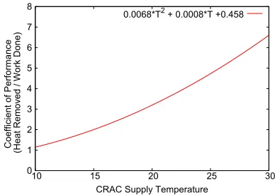
CRAC Supply Temperature 0.0068*T2+ 0.0008*T +0.458

Fig. 8. Typical model of the Coefficient of Performance (COP) curve for a chilled water CRAC unit.

Hewlett-Packard’s Proliant DL360 G3s model, which consumes 150W of power when idle and 285W at 100% utilization. From this we can determine that the total power consumption of the data centre is168kW when idle and319.2kW at full utilisation. For cooling, the data centre is equipped with four CRAC units. Each CRAC unit pushes air chilled to 15◦C into the plenum at a rate of16,990m_h3. The cooling capacity of the each CRAC unit is limited to 90kW, and in full operation each CRAC unit itself consumes10kW.

The layout of the two data centres modelled is shown in Figure 7. Racks of servers are represented as boxes with the letter “S” and CRAC units can be iden-tified as boxes with the letter “C”. The simulations are used to establish the maximum inlet temperature of a server rack Tmax. We can use this to establish the

cooling costsC which can be calculated as follows:

C= Q

COP(Tsup+ (Tsaf e−Tmax))

+Pf an (1)

Where Q is the amount of power the servers con-sume,Tsup the temperature of the air that the CRAC

units supply,Tsaf ethe maximum permissible

temper-ature at the server inlets in order to prevent equip-ment damage, Tmax the maximum temperature of

the server inlets in the data centre, Pf an the power

required by the fans of the CRAC units and COP is the “coefficient of performance” (COP), that is the ratio of heat removed to work necessary to remove the heat, is a function of the temperature of the air being supplied by the CRAC unit. The COP of a typical chilled-water CRAC unit used in the calculations of cooling costs is depicted in Figure 8. We assume aTsaf evalue of25◦C.

AC

C

C

C

S S S S S S S

S S S S S S S

AC

C

C

C

S S S S S S S

S S S S S S S

S S S S S S S

S S S S S S S

Co

ld

A

isle

Co

ld

A

isle

Ho

t A

isl

e

(a) Cold Aisle Containment (b) No Cold Aisle Containment S

S S S S S S

S S S S S S S

Co

ld

A

isle

Co

ld

A

isle

Ho

t A

isl

e

Fig. 7. Layout of cooling cost simulations with (a) cold aisle containment and (b) no cold aisle containment.

TABLE 1

Average round trip time between data centres and sources of requests, carbon intensity of data centres and sources of requests and daily number of requests at source

Region California (ms) Ireland (ms) Virginia (ms) Carbon Intensity

(g/kWhr)

Number of Requests

(Millions)

Austria (AUS) 177.98 47.67 159.07 870 7.038

Belgium (BEL) 171.98 28.45 158.09 317 11.736

California (CAL) 384

Colorado (COL) 42.77 155.36 101.27 903 6.76

Connecticut (CON) 88.05 117.65 75.73 392 4.293

Finland (FIN) 188.47 55.77 176.72 99 5.418

Florida (FLO) 54.26 171.87 98.21 762 26.365

France (FRA) 192.44 21.24 184.75 96 61.355

Georgia (GEO) 58.91 115.12 77.43 694 1.968

Germany (GER) 177.74 40.89 157.68 612 58.76

Illinois (ILL) 63.81 142.78 102.08 544 18.049

Indiana (IND) 69.65 151.05 83 986 7.803

Ireland (IRE) 655

Italy (ITA) 188.71 44.71 167.3 473 55.372

Kansas (KAN) 50.48 148.4 85.2 817 4.545

Kentucky (KEN) 71.98 146.85 87.29 968 5.169

Maryland (MAR) 99.71 140.46 88.05 641 6.69

Massachusetts (MAS) 89.33 98.02 72.1 603 9.602

Minnesota (MIN) 62.09 147.74 85.79 744 6.724

Netherlands (NET) 163.93 19.71 138.79 548 15.527

New York (NEW) 96.45 78.71 134.11 386 27.604

North Carolina (NCA) 72.32 72.45 31.12 604 11.817

Norway (NOR) 194.82 48.84 183.08 6 6.69

Ohio (OHI) 83.81 132.08 69.17 873 14.828

Oklahoma (OKL) 46.42 159.96 98.22 819 4.378

Ontario (ONT) 90.84 142.81 97.12 224 16.64

Oregon (ORE) 27.66 213.48 153.28 246 4.807

Pennsylvania (PEN) 71.99 118.53 52.78 597 16.097

Portugal (POR) 222.69 64.11 190.02 550 10.925

Spain (SPA) 194.55 35.83 172.47 487 40.633

Sweden (SWE) 186.01 48.79 170.28 19 11.887

Tennessee (TEN) 235.61 276.43 311.61 661 7.891

Texas (TEX) 37.61 151.93 98.96 763 31.015

UK (UK) 175.59 17.62 163.25 614 78.647

Virginia (VIR) 559

Washington (WAS) 29.57 192.11 126.53 938 10.119

0 50000 100000 150000 200000 250000 300000

0 20 40 60 80 100

Cool

ing Costs (W)

Percentage Total Demand CAC-CRAC

NCAC-CRAC FAC

Fig. 9. Cooling cost of various data centre cooling systems at various levels of demand

cold aisle containment and CRAC cooling. “Free air cooling ” only consumes fan power and is therefore constant.

5.4 Average Job Time

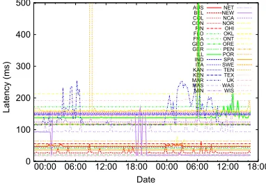
The previous sections establish that electricity cost and carbon emissions can be lowered. It is likely, however, that there will be an increase in the average service request time which the cloud operator will have to take into account when determining its load balancing policy. A useful metric for service request time is the latency between the server and client. To establish the round trip time data an experiment on PlanetLab [39] was established with a server at each node location. Nodes in the same region as our three data centre locations then pinged the other geographical regions at fifteen minute intervals for approximately two days. The average latency estab-lished from this experiment can been seen in Table 1. Average service request time could be reduced by routing load from a geographical region to the data centre region using lowest latency as a criterion to route load. From Table 1 we can see that if such a load balancing scheme was used, each data centre region will have some of the load routed to it. From this we can conclude that any reduction in carbon emissions or electricity cost will cause an increase in the average latency as load will not be routed with latency as the sole metric.

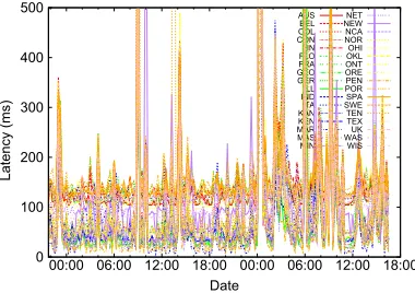
Figure 10, 11 and 12 depict the measured latency between the data centre and the other regions for the California, Ireland and Virginia data centres re-spectively. It is interesting to note that the latencies remain mostly constant over time at the California and Ireland data centres but vary frequently at the Vir-ginia data centre. We postulate that this is a result of congestion at the Virginia region. In addition, we can see that there is some variation in the latency between the other regions and the California and Ireland data centres. Thus we can conclude that latency varies with time particularly in regions where congestion takes

0 100 200 300 400 500

00:00 06:00 12:00 18:00 00:00 06:00 12:00 18:00

Latency (ms)

Date

AUS BEL COL CON FIN FLO FRA GEO GER ILL IND ITA KAN KEN MAR MAS MIN

NET NEW NCA NOR OHI OKL ONT ORE PEN POR SPA SWE TEN TEX UK WAS WIS

Fig. 10. Latency between California and different geographical regions at fifteen minute intervals.

0 100 200 300 400 500

00:00 06:00 12:00 18:00 00:00 06:00 12:00 18:00

Latency (ms)

Date

AUS BEL COL CON FIN FLO FRA GEO GER ILL IND ITA KAN KEN MAR MAS MIN

NET NEW NCA NOR OHI OKL ONT ORE PEN POR SPA SWE TEN TEX UK WAS WIS

Fig. 11. Latency between Ireland and different geo-graphical regions at fifteen minute intervals.

place and it should be monitored so that the increase in average service request time caused by reducing carbon emissions or electricity cost can be measured correctly. Indeed there may be times, where there is no increase in average service request time associated with a reduction in carbon emissions or electricity cost.

6

S

S

In this section we describe the setup for the simu-lation of the algorithm described in Section 4 and our methodology for establishing the weights of the graph described in Section 3.4. We simulate three data centres. One of these in Ireland and the other two are in the United States in Virginia and California. We chose these locations to mimic Amazon’s EC2 platform [27] which currently has major data centres at these locations. We model 34 sources of requests in the simulation which represent certain countries in Europe, states in the United States and provinces in Canada. Each source is connected to each data centre by a single edge. This is illustrated in Figure 13.

Fig. 13. Diagram of the simulation setup. The colour of the node indicates that the node is part of a particular partition.

0 100 200 300 400 500

00:00 06:00 12:00 18:00 00:00 06:00 12:00 18:00

Latency (ms)

Date

AUS BEL COL CON FIN FLO FRA GEO GER ILL IND ITA KAN KEN MAR MAS MIN

NET NEW NCA NOR OHI OKL ONT ORE PEN POR SPA SWE TEN TEX UK WAS WIS

Fig. 12. Latency between Virginia and different geo-graphical regions at fifteen minute intervals.

For the networking portion of a request, we firstly assume that each service request requires the transfer of relatively small amount of data and therefore the duration of the connection can be approximated by the round trip time. To calculate the time associated with the computational portion of the request we assume that the request requires50ms of computation. In order to calculate the carbon emissions and electricity cost of serving a request we assume that the data centre uses Hewlett-Packard’sProliant DL360 G3s. This type of server consumes 150W at 0% util-isation and 285W at 100% utilization. This yields dynamic power of 135W for each server. This is then multiplied by the time required to service the computational portion of the request (50ms) to yield the energy required to service a request. We must then consider the energy required for the additional cooling required by servicing the requests. We assume that the Ireland data centre uses “free air cooling”, the Virginia data centre uses cold aisle containment and the California data centre uses a standard cooling system with no cold aisle containment. The cooling energy required by the data centre when it is not

processing the request is subtracted from the energy required when it is processing the request to give the cooling energy caused by the request. This is added to the energy already calculated to yield the total computational energy. The total computational energy is then multiplied by the electricity price to yield the electricity cost Ei. The energy is also multiplied by

the carbon intensity of the data centre to yield the computational carbon emitted.

The networking aspect of the weights must also be considered. The power consumed by a switch can be altered by powering off (disabling) ports when they are not in use and powering on (enabling) ports when they need to be used. In order to calculate the carbon emissions associated with servicing the networking portion of the request we assumed that only two ports would open during the duration of the request. To calculate the carbon emitted we first obtain the energy consumed by multiplying the duration of the round trip by a power value required to open a port (0.7W). This value was an intermediate value of those presented in [20]. The energy consumed is then multiplied by the average carbon intensity of the source of the request and the data centre to obtain the network carbon emitted. This is added to the computational carbon emitted to give the total carbon emitted and the carbon weightGi. While cloud

oper-ators are likely to be held at least partially responsible for the carbon emissions of the networking aspect by increased regulation, current modes of operation suggest that they are not held responsible for the vast majority of the electricity cost of this aspect and as such it is ignored.

centres. The carbon intensity data is as seen in Table 1 for all the regions except Ireland which uses the data seen in the first two days of Figure 6. The algorithm updates every fifteen minutes. It is assumed that the time required to service a request is sufficiently short that redirection is not required to minimize the cost when the algorithm updates. It should be noted that we assume that redirecting additional requests to each data centre does not cause congestion or affect the average service request time.

In order to examine the overall costs to the cloud we must consider the number of requests coming from each source of requests. We used figures from the websites [40], [41] which estimated the number of Facebook users in each source location and assumed that the daily average number of service requests from a single user was 2.6. We used Facebook as it is representative of a broad range of cloud applica-tions. The daily number of requests for each source can be seen in Table 1. We also needed to establish the number of requests at each source during each fifteen minute interval over the two day period. It has previously been found that realistic workloads have a diurnal cycle with a trough at approximately 6:00am and a peak of roughly four times the trough value at approximately midnight [1]. We divided the daily number of requests at each source into this diurnal pattern and adjust the peaks to match the time difference of the region. The total demand can be seen in Figure 14.

In the first set of simulation we examine the ex-tremes of the algorithm by looking at four scenar-ios. In the first scenario we set the relative price functions to zero. This represents a scenario where time is crucial and the operator is attempting to minimize the time taken to service a request with no regard for electricity cost and associated carbon emissions R1(Gi) = 0, R2(Ei) = 0 and the weights

of the edges of the graph become wi =Ti. We shall

hereafter refer to this scenario as “Best Effort Time”. In the second scenario we set the first relative price function to ten thousand times the carbon emissions. This essentially functions as infinite times the carbon emission. This represents a scenario where time and electricity cost are unimportant and all efforts can be made to reduce the associated carbon emissions R1(Gi) = 10000Gi, R2(Ei) = 0 and the weights of the

edges of the graph becomewi=Ti+10000Gi. We shall

hereafter refer to this scenario as “Best Effort Carbon”. In the third scenario we set the second relative price function to ten thousand time the electricity cost. This represents a scenario where time and carbon emissions are unimportant and all efforts can be made to lower the electricity costs R1(Gi) = 0, R2(Ei) =

10000Ei and the weights of the edges of the graph

become wi = Ti + 10000Ei. We shall hereafter refer

to this scenario as “Best Effort Electricity”. In the final scenario we examine a baseline for current load

balancing operations by examining a round robin scheme. This is the default option in many commercial load balancing solutions. We shall hereafter to refer to this scenario as “RoundRobin”.

In the second set of simulations we explore scenar-ios where the cloud operator needs to strike a balance between the three factors. In this set of simulations we examine the performance of the algorithm under scenarios which attempt to balance the various factors by adjusting (α, β) R1(Gi) = αGi, R2(Ei) = βEi in

intervals of 100 from 0 to 10000 and examining the total electricity cost, carbon emissions and average service request time of each scenario to examine what savings in electricity cost and carbon emissions can be made when there are constraints on the average service request time. We defineαas a variable which represents the relative importance of carbon emissions to the cloud operator and β as a variable which represents the relative importance of electricity cost.

7

R

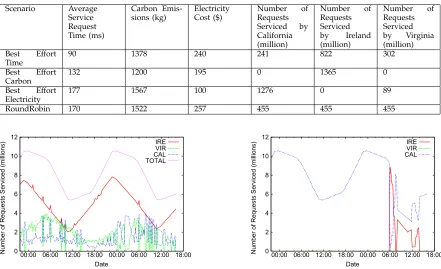
The key performance metrics for the simulations are the average service request time, the electricity cost and the carbon emissions associated with servicing requests for the two days. We first examine these for the first set of simulations. They are shown for each scenario in Table 2. When comparing the best effort carbon scenario with the roundrobin baseline we can see that carbon emissions for a service can be reduced by 21%. If we examine the best effort electricity scenario and the roundrobin baseline we can see that the electricity cost can be reduced by 61%. There is, however, a corresponding increase in the average service request time of 7ms. If we investi-gate the best effort time scenario and the roundrobin baseline we can see that the average service request time can be reduced by 47%. It is also interesting to compare the three best effort scenarios. If we compare the best effort time scenario and the best effort carbon scenario we see that the latter emits 13% less carbon but has an average service request time that is 42ms higher. If we examine the best effort time scenario and the best effort electricity scenario we can see that the latter costs 58% less but has an average service request time that is 87ms higher. These comparisons are useful for the cloud operator as it allows them to see if the scenarios are feasible under SLAs and whether it is more desirable to concentrate on lower electricity costs or carbon emissions.

TABLE 2

Average Service Request time, Daily Carbon Emission and Number of Requests Serviced at Each DC for Various Scenarios

Scenario Average

Service Request Time (ms)

Carbon Emis-sions (kg)

Electricity Cost ($)

Number of

Requests

Serviced by

California (million)

Number of

Requests Serviced

by Ireland

(million)

Number of

Requests Serviced

by Virginia

(million)

Best Effort

Time

90 1378 240 241 822 302

Best Effort

Carbon

132 1200 195 0 1365 0

Best Effort

Electricity

177 1567 100 1276 0 89

RoundRobin 170 1522 257 455 455 455

0 2 4 6 8 10 12

00:00 06:00 12:00 18:00 00:00 06:00 12:00 18:00

Numbe

r

of

Re

quests S

erviced

(mi

llions)

Date

IRE VIR CAL TOTAL

Fig. 14. Number of requests serviced at each data centre when the “Best Effort Time” scenario is used. It shows UTC local time.

0 2 4 6 8 10 12

00:00 06:00 12:00 18:00 00:00 06:00 12:00 18:00

Numbe

r

of

Re

quests S

erviced

(mi

llions)

Date

IRE VIR CAL

Fig. 15. Number of requests serviced at each data centre when the “Best Effort Carbon” scenario is used. It shows UTC local time.

centre under this scenario. We can also see that under the best effort electricity scenario most of the load goes the California data centre. It is interesting that the additional electricity cost of the cooling setup in the data centre is mostly insufficient to overcome the local electricity price differential and the requests mostly go to the California data centre. We also examine the number of requests serviced at the data centres at each time interval. Figure 14 depicts the numbers of requests serviced at each data centre during a

0 2 4 6 8 10 12

00:00 06:00 12:00 18:00 00:00 06:00 12:00 18:00

Numbe

r

of

Re

quests S

erviced

(mi

llions)

Date

IRE VIR CAL

Fig. 16. Number of requests serviced at each data centre when the “Best Effort Electricity” scenario is used. It shows UTC local time.

0 2 4 6 8 10 12 14

00:00 06:00 12:00 18:00 00:00 06:00 12:00 18:00

Carbon Emitted (kg)

Date

BE-CAR BE-ELE BE-TIM RR

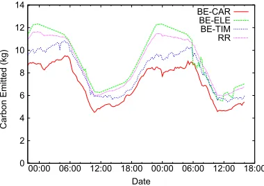
Fig. 17. Carbon Emitted at each time interval under a variety of scenarios. It shows UTC local time.

0 0.5 1 1.5 2 2.5 3

00:00 06:00 12:00 18:00 00:00 06:00 12:00 18:00

Electricity cost ($)

Date

BE-CAR BE-ELE BE-TIM RR

Fig. 18. Electricity Cost at each time interval under a variety of scenarios. It shows UTC local time.

to the Ireland data centre. Finally all the requests get serviced by the California data centre as the prices diverge.

Figure 17 depicts the carbon emitted under each scenario over the time period. From Figure 17 we can see that the carbon emitted follows the number of service requests under all scenarios. This is as we expected as more service requests require more energy which increases the carbon emissions. We can also see there are no spikes in the emissions which is as we expected as Figure 6 shows that the change in carbon intensity over time is gradual. Finally we can see that the difference between the schemes is quite small. The carbon intensities of the three data centres are relatively similar. The Ireland data centre’s car-bon intensity ranges from 369g/kWhr to 522g/kWhr, Virginia has a carbon intensity of 559g/kWhr and California has a carbon intensity of 384g/kWhr but this is offset by the cooling setup used in our simu-lation data centre. The difference in carbon intensities between other regions is much larger. For example Norway with its high level of hydropower has a carbon intensity of 6g/kWhr while Austria has a carbon intensity of 870g/kWhr.

Figure 18 depicts the electricity cost under each scenario over the time period. From Figure 18 we can

0 50 100 150 200 250 300 350 400

00:00 06:00 12:00 18:00 00:00 06:00 12:00 18:00

Average

Se

rvice Requ

est Time (ms)

Date

BE-CAR BE-ELE BE-TIM RR

Fig. 19. Average service request time at each time interval under a variety of scenarios. It shows UTC local time.

see that the difference between the various scenarios can be quite large particularily when there are peaks in the electricity cost at the data centre where requests are being serviced. It is also interesting to note that the difference can be quite small as we can see that the electricity cost of the best effort carbon scenario and the best effort electricity scenario are effectively the same towards the end of the time period. It should be noted that the while the overall electricity cost is quite low it is the relative differences in the electricity price that are the most important. In our model we assumed that a single server performs all the computation required for a single request. While it is possible for cloud services to use this approach, latency considera-tion frequently result in a Particonsidera-tion/Aggregate design pattern being used [42]. In this approach a request is broken into pieces which are then farmed out to worker servers. The responses of the workers are aggregated together by aggregator servers to yield the result to the request. In this design hundreds of servers can be used to process a single request although typically tens of servers are used to handle requests. In this design the energy consumption for a request is significantly higher as tens of servers are operating simultaneously and the overall electricity cost would consequently be significantly higher. We chose not to model the requests in this fashion as without trace data it is difficult to simulate this design accurately as each worker server frequently operates for different lengths of time and therefore the energy consumed by each worker will be different.

0

2000 4000

6000 8000₁₀₀₀₀₀20004000 60008000

10000 0

200 400 600 800 1000 1200 1400 1600

Total carbon emitted (k

g)

α

β

Total carbon emitted (k

g)

1200 1250 1300 1350 1400 1450 1500 1550 1600

Fig. 20. Total carbon output with varying relative price functions.

0

2000 4000

6000 8000₁₀₀₀₀₀20004000 60008000

10000 0

50 100 150 200 250 300

Total electricity cost ($)

α

β

Total electricity cost ($)

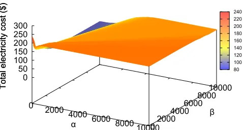
80 100 120 140 160 180 200 220 240

Fig. 21. Total electricity cost with varying relative price functions.

demand in the regions. If there are more requests in from a region with high latency at a given time interval this will increase the average service request time. This does not occur in the roundrobin and best effort time scenarios as the requests are spread among the three data centres and the effect is diluted. It is important that the cloud operator considers this so that SLAs are not violated.

We now examine the second set of simulations. Figure 20 depicts the total carbon output as we vary α and β. From Figure 20 we can see that as we increase α the carbon emissions decrease and that as we increase β the total carbon emissions increase. Figure 21 depict the total electricity cost as we vary α and β. From Figure 21 we can that we increase α the electricity cost increases and as we increase β the electricity cost decreases. Figure 22 depicts the average service request time as we varyαandβ. From Figure 22 we can see that as we increase αand β we increase the average service request time. The increase is more severe in β’s case but this is a result of the particulars of the simulations as the average latency between all the regions and the California data centre is higher than the average latency between all the regions and the Ireland data centre. Figure 21 is not monotonic as the initial increase of αfrom zero will move requests from Virginia to Dublin which lowers the electricity cost while increasing α beyond this

0

2000 4000

6000 8000

1000002000 40006000

800010000 0

20 40 60 80 100 120 140

Average

Se

rvice Requ

est Time (ms)

α

β

Average

Se

rvice Requ

est Time (ms)

90 100 110 120 130 140 150

Fig. 22. Average service request time with varying relative price functions.

point moves requests from California to Dublin which increases the overall electricity cost. Similar trends can be seen in Figure 22.

The selection ofα andβ are of crucial importance to the operation of this algorithm. Ultimately the selection of these values will depend on the SLAs the cloud operator has agreed to. Savings in electricity cost and reductions in carbon emissions can only be achieved if SLAs can still be maintained while there is an increase in the average service request time. The selection of whether to lower carbon emissions or electricity cost will depend on whether the cloud operator is under any regulation to limit its carbon emissions, public relations pressures or the price of carbon on carbon trading schemes. The first set of simulations has shown the average service request time will vary with time. From this we can conclude that α and β will also vary with time. It would, however, be relatively simple to alter the algorithm so thatαand β are adjusted at each time interval in relations to the average service request time of the previous time interval and this is left for future work.

8

C

A

This work is partially funded by the Irish Higher Education Authority under the HEA PRTLI Network Mathematics Grant and by SFI grant 07/IN.1/I901.

R

[1] A. Qureshi, J. Guttag, R. Weber, B. Maggs, and H. Balakrish-nan, “Cutting the electric bill for internet-scale systems,” in

Proceedings of ACM SIGCOMM, Barcelona, 17-21 August 2009, pp. 123–134.

[2] R. Stanojevi´c and R. Shorten, “Distributed dynamic speed scaling,” in Proceedings of IEEE INFOCOM, San Diego, 14-19 March 2010, pp. 1–5.

[3] Z. Liu, M. Lin, A. Wierman, S. H. Low, and L. L. Andrew, “Greening geographical load balancing,” inProceeding of SIG-METRICS, San Jose, 7 June 2011, pp. 233–244.

[4] M. Conti, E. Gregori, and F. Panzieri, “Load distribution among replicated Web servers: a QoS-based approach,” SIG-METRICS Performance Evaluation Review, vol. 27, no. 4, pp. 12– 19, 2000.

[5] Z. M. Mao, C. D. Cranor, F. Bouglis, M. Rabinovich,

O. Spatscheck, and J. Wang, “A precise and Efficient Evalu-ation of the Proximity between Web Clients and their Local DNS Servers,” in Proceedings of USENIX, Monterey, 10 - 15 June 2002, pp. 229–242.

[6] M. Pathan, C. Vecchiola, and R. Buyya, “Load and Proximity Aware Request-Redirection for Dynamic Load Distribution in Peering CDNs,” inOn the Move to Meaningful Internet Systems: OTM, ser. Lecture Notes in Computer Science. Springer Berlin / Heidelberg, 2008, vol. 5331, pp. 62–81.

[7] Greenpeace, “Make IT green cloud computing and its

contribution to climate change,” Retrieved February 2011, http://www.greenpeace.org/international/Global

/international/planet-2/report/2010/3/make-it-green-cloud-computing.pdf.

[8] I. B. Fridleifsson, R. Bertani, E. Huenges, J. W. Lund, A. Rag-narsson, and L. Rybach, “The possible role and contribution of geothermal energy to the mitigation of climate change,”

O. Hohmeyer and T. Trittin (Eds.) IPCC Scoping Meeting on Renewable Energy Sources. Proceedings, pp. 59–80, 2008. [9] M. Lenzen, “Life cycle energy and greenhouse gas emissions of

nuclear energy: A review,”Energy Conversion and Management, vol. 49(8), pp. 2178–2199, August 2008.

[10] “European Union Emissions Trading System,”

http://ec.europa.eu/clima/policies/ets/.

[11] chuangang Ren, D. Wang, B. Urgaokar, and A. Sivasubrama-niam.

[12] Z. Liu, M. Lin, A. Wierman, S. H. Low, and L. L. Andrew, “Geographical load balancing with renewables,” inProceeding of GreenMETRICS, San Jose, 7 - 11 June 2011, pp. 1–5. [13] J. Doyle, D. O’Mahony, and R. Shorten, “Server selection for

carbon emission control,” in Proceeding of ACM SIGCOMM Workshop on Green Networking, Toronto, 19 August 2011, pp. 1–6.

[14] J. Baliga, R. W. A. Ayre, K. Hinton, and R. S. Tucker, “Green cloud computing: Balancing energy in processing, storage, and transport,”Proceeding of the IEEE, vol. 99(1), pp. 149–167, 2011. [15] J. W. Durham, R. Carli, P. Frasca, and F. Bullo, “Discrete Partitioning and Coverage Control for Gossiping Robots,”

IEEE Transactions on Robots, vol. 28, no. 2, pp. 364–378, 2012. [16] L. Rao, X. Liu, L. Xie, and W. Liu, “Minimizing electricity

cost: Optimization of distributed internet data centers in a multi-electricity-market environment,” inProceedings of IEEE INFOCOM, San Diego, 15 - 19 March 2010, pp. 1–9.

[17] L. Rao, X. Liu, M. D. Ilic, and J. Liu, “Distributed Coordina-tion of Internet Data Centers Under Multiregional Electricity Markets,”Proceedings of the IEEE, vol. 100, no. 1, pp. 269–282, 2012.

[18] P. Wang, L. Rao, X. Liu, and Y. Qi, “D-Pro: Dynamic Data Center Operations With Demand-Responsive Electricity Prices in Smart Grid,”IEEE Transactions on Smart Grid, vol. 3, no. 4, pp. 1743–1754, 2012.

[19] V. Mathew, R. K. Sitaraman, and P. Shenoy, “Energy-aware load balancing in content delivery networks,” inProceedings of IEEE INFOCOM, Orlando, 25 - 30 March 2012, pp. 954–962. [20] P. Mahadevan, S. Banerjee, and P. Sharma, “Energy propor-tionality of an enterprise network,” in Proceedings of ACM GreenNet, New Delhi, 30 August 2010, pp. 53–60.

[21] F. F. Moghaddam, M. Cheriet, and K. K. Nguyen, “Low Carbon Virtual Private Clouds,” in Proceedings of IEEE International Conference on Cloud Computing, Washington DC, 4 - 9 July 2011, pp. 259–266.

[22] P. X. Gao, A. R. Curtis, B. Wong, and S. Keshav, “It’s not easy being green,” in Proceedings of SIGCOMM, Helsinki, 13 - 17 August 2012, pp. 221–222.

[23] F. Aurenhammer, “Voronoi Diagrams-a survey of a fundamen-tal geometric data structure,”ACM Computing Surveys, vol. 23, no. 3, pp. 345–405, September 1991.

[24] R. J. Fowler, M. S. PAterson, and S. L. Tanimoto, “Optimal packing and covering in the plane are NP-complete,” Informa-tion processing letters, vol. 12, pp. 133–137, 1981.

[25] R. Z. Hwang, R. C. T. Lee, and R. C. Chang, “The slab dividing approach to solve the Euclidean p-center problem,”

Algorithmica.

[26] T. F. Gonzalez, “Clustering to minimize the maxium interclus-ter distance,”Theoretical Computer Science, vol. 38, pp. 293–306, 1985.

[27] Amazon, “Elastic Compute Cloud,”

http://aws.amazon.com/ec2.

[28] “Carbon Monitoring for Action,” http://carma.org/.

[29] United States Environmental Protection Agency,

“eGRID,”

http://www.epa.gov/cleanenergy/energy-resources/egrid/index.html. [30] Eirgrid, http://www.eirgrid.com.

[31] Mikko Pervil¨a and Jussi Kangasharju, “Cold air containment,” inProceedings of ACM SIGCOMM Workshop on Green Network-ing, Toronto, 19 August 2011, pp. 7–12.

[32] L. A. Barroso and U. H ¨olzle, “The datacenter as a computer: An introduction to the design of warehouse-scale machines,”

Synthesis Lectures on Computer Architecture, 2009.

[33] D. Atwood and J. G. Miner, “Reducing data

center cost with an air economizer,” August 2008,

http://www.intel.com/content/www/us/en/data-center- efficiency/data-center-efficiency-xeon-reducing-data-center-cost-with-air-economizer-brief.html.

[34] P. Rumsey, “Overview of liquid cooling systems,” 2007,

http://hightech.lbl.gov/presentations/Dominguez/5 LiquidCooling 101807.ppt. [35] A. Almoli, A. Thompson, N. Kapur, J. Summers, H. Thompson,

and G. Hannah, “Computational fluid dynamic investigation of liquid rack cooling in data centres,”Applied Energy, vol. 89, pp. 150–155, 2012.

[36] M. G. Corporation, “Flovent version 9.1,” Wilsonville, Oregon, USA, 2010.

[37] R. K. Sharma, C. E. Bash, and C. D. Patel, “Balance of power: Dynamic thermal management for internet data centers,”IEEE Internet Computing, vol. 9(1), pp. 42–49, 2005.

[38] J. Moore, J. S. Chase, P. Ranganathan, and R. Sharma, “Making scheduling “Cool”: Temperature-aware workload placement in data centers,” in Proceedings of USENIX, Anaheim, 10-15 April 2005, pp. 61–75.

[39] B. Chun, D. Culler, T. Roscoe, A. Bavier, L. Peterson, M. Wawr-zoniak, and M. Bowman, “PlanetLab: an overlay testbed for broad-coverage services,”SIGCOMM Computer Communication Review, vol. 33, no. 3, pp. 3–12, 2003.

[40] Social Bakers, “Social bakers the recipe for social marketing success,” http://www.socialbakers.com/facebook-statistics/. [41] Internet World Stats, “Internet world stats usage and

popula-tion statistics,” http://www.internetworldstats.com.