Influence of Growth of Reeds on Evapotranspiration in
Horizontal Subsurface Flow Constructed Wetlands
Tokuo Yano
1,*, Masatomo Nakayama
2, Kazuhiro Yamada
1, Akiko Inoue-Kohama
1,
Shinya Sato
3, Keijiro Enari
11Department of Environment and Energy, Tohoku Institute of Technology, Japan 2Department of Civil Engineering and Management, Tohoku Institute of Technology, Japan
3Sendai Kankyo Kaihatsu Co., Ltd, Japan
Copyright©2017 by authors, all rights reserved. Authors agree that this article remains permanently open access under the terms of the Creative Commons Attribution License 4.0 International License
Abstract
In this study, the influence of growth of reeds on evapotranspiration (ET) was estimated, and a commonly used meteorological estimate of potential evapotranspiration (PET) was compared with direct measurements of ET. The salinity of the inside of HSF of the raw leachate inflow was 15.0±3.4g Cl-/L and that of the double diluted inflow was 9.3±1.9g Cl-/L. Although the growth of reeds in the raw leachate inflowwas impeded remarkably compared to that of the double diluted leachate inflow, the reeds in the double diluted inflow bed showed healthy growth. The difference in the salinity gave rise to large differences in the growth of the reed. The annual ET rates in the poor vegetation bed, the dense vegetation bed and the unplanted bed were 656.5mm, 2,334.3mm and 22.2mm, respectively. The difference of the growth of the reed provided a large difference in the ET rate. The annual PET estimated on the basis of the Hamon equation was 751.6mm. The PET rate was much lower compared to the ET rate in the dense vegetation bed. It was necessary to consider site-specific factors such as the growth of plants in the evaluation of the water budget in the HSFs.Keywords
Evapotranspiration, Growth of Reeds, HSF, Potential Evapotranspiration, Water Budget1. Introduction
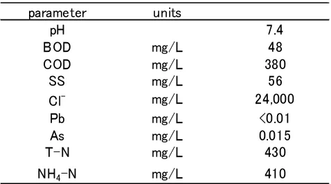
In Japan, most waste is incinerated in order to reduce the landfill disposal of wastes and the incinerated ashes are dumped into landfills. As the ashes contain a large quantity of inorganic salts, most landfill-leachates contain a high salinity which is higher than that of sea water. Table1 shows an example of the landfill- leachate quality.
Plants are an important component of constructed wetlands. Although various kinds of plants such as reed, reed canary glass, cattail, papyrus, iris, etc., are planted in the constructed wetlands [1], a high salinity remarkably impedes
the growth of many plants. It is assumed, however, that reeds can tolerate a high degree of salinity. Matoh demonstrated that reeds were successfully grown at chloride concentrations of up to17.8g・Cl-/L, and reeds could grow
normally until 10.7g・Cl-/L [2]. Barr reported that P.
australis could tolerate salinity to quite a high degree of up to 7.3g・Cl-/L for normal growth, surviving at up to 12.7g・
Cl-/L [3]. Mauchamp demonstrated that reed growth decreased as salinity increased (50% decrease at 4.6g・Cl-/L
when compared to freshwater) and a 7-100% mortality depending on population, occurred at 9.1g・Cl-/ L and 12.1g ・Cl-/L[4].
Table 1. Landfill-leachate quality
Although, there were few studies concerning the treatment of high salinity landfill-leachate with constructed wetlands, some reports concerning horizontal subsurface constructed wetlands (HSFs) were given over the past several years [5-8].
There are several roles of wetland plants on constructed wetlands [9-11],: (1) prevention of clogging by rhizome of plants, (2) oxygen release from the rhizome, (3) the offer of a habitat of a rhizosphere, (4) uptake of nutrients, and (5) the offer of a natural landscape.
Vymazal and Kropfelva published literature reviews on the role of plants in HSF [1]. However, the mechanisms by
parameter units
pH 7.4
BOD mg/L 48
COD mg/L 380
SS mg/L 56
Cl- mg/L 24,000
Pb mg/L <0.01
As mg/L 0.015
T-N mg/L 430
[image:1.595.312.551.469.602.2]which macrophytes affect water treatment in constructed wetlands are under debate. Evapotranspiration is one of the most important roles of plants. Constructed wetlands receive water through inflows and precipitation, and lose water to outflows, evaporation and transpiration, i.e., evapotranspiration (ET). The evapotranspiration of plants has a close relation to the water budget in the constructed wetlands and influences the HRT and purification process [12]. Plants have a critical role in determining the dynamics of water loss, mainly through ET. There have been many studies concerning the ET of constructed wetlands, and these studies demonstrate that the ET of emergent macrophytes is a significant process in constructed wetlands [13-15]. For example, ET from a constructed wetland in Morocco planted with Arundo donax was 40mm/d and 60mm/d with Phragmites australis, compared to 7mm/d in an unplanted HSF [14].
However, there have been few studies concerning the influence of growth of reeds on ET up to now. Difficulties in accurately calculating ET in constructed wetlands may lead to inaccurate water balance [15]. Simple meteorological methods or off-site ET data often are used to estimate, but these approaches do not include potentially important site specific factors such as plant communities, root zones, water levels, and soil properties.
The objective of this study was to estimate the influence of growth of reeds on ET and to compare a commonly used meteorological estimate of potential evapotranspiration (PET) with the ET, which is estimated on the basis of water balance method.
2. Materials and Methods
2.1. Materials
Reeds grown under high salinity conditions had higher treatment efficiencies than reeds grown under low salinity conditions in the treatment of high salinity landfill leachate [5]. Therefore, in this study, the reeds which vegetated around the estuary area of the mouth of the Nanakita River located at the eastern part of Sendai City were used. Six stocks of reed were planted in a bed on April 2010 and the experiment was started.
2.2. Experimental Designs
The pilot-scale HSFs were located in Miyagi Prefecture in Japan. The experimental approaches consisted of three runs: Run A was a raw leachate inflow with reeds, Run B was a double diluted leachate inflow with reeds and Run C was a double diluted leachate inflow without reeds. The three pilot-scale constructed wetlands were identical in size and construction (2m long × 1m wide with a water depth of 0.55m). Inflow, outflow and precipitation were measured in order to evaluate the water budget of the constructed
wetlands.
The schematic diagram of the pilot scale HSFs is shown in Figure 1.
Figure 1. Schematic diagram of apparatus; (a) Configuration of HSFs; (b) Longitudinal view of apparatus
Figure 1-a is a configuration of HSFs.
The flow rate was 50L/day, giving a theoretical HRT of 10 days. Five sampling wells constructed to enable water extraction from the upper, middle and lower layers of the water column were placed at equal intervals between the inlet and outlet devices. The wells corresponded to the theoretical residence times of 1.8, 3.6, 5.0, 6.4 and 8.2 days if the plug flow through the bed is assumed. The sampling points and HRT of the apparatus are shown in Figure 1-b. The salinity of the sampling point of 3-2 in the Figure 1-b was assumed as the representative of the salinity of inside of the HSF.
the Hamon equation.
The meteorological data were collected during experiments using a weather station located adjacent to the HSF units.
3. Results and Discussions
3.1. Salinity of the inside of Constructed Wetlands Figure 2 shows the variation of the inflow salinity of Run A and Run B, the salinity of the inside of HSFs and the total of the 10 day-precipitation just before the measurement of salinity inside of the HSFs during the period from January 2010 to December 2014. As the HRT of HSF is 10 days, the 10-day precipitation is shown in the figure.
The salinity of Run A inflow was within the range of 12.8
to 23.6g・Cl-/L, with an average of 19.1±2.2 g・Cl-/L. That
of the Run B inflow was within the range of 4.3 to 14.7g・
Cl-/L , with an average of 10.4±1.9g・Cl-/L. The salinity of Run B inflow had been doubly diluted compared to that of Run A inflow during the experimental periods.
The salinity of the inside of Run A varied from 4.8 to 20.7 g・Cl-/L, with an average of 15.0±3.4 g・Cl-/L. That of Run
B varied from 3.5 to 13.7g・Cl-/L, with an average of
9.3±1.9 g・Cl-/L. The high precipitation reduced the salinity
inside of the HSFs. The salinity of the survival limit of a reed is reported within the range of 12-15g・Cl-/L[4,5]. As shown
in Figure 2, the salinity of the inside of Run A was 15.0±3.4g Cl-/L and that of Run B was 9.3±1.9g Cl-/L. The reeds of Run A had a difficulty remaining alive under the salinity conditions of Run A. On the other hand, the reeds of Run B are able to survive under the salinity conditions of Run B.
Figure 2. Salinity of inside of HSFs and precipitation
Figure 3. Seasonal growth change of reeds (2014): (a) Shoot length (n of Run A: 30, n of Run B: 30) and (b) Shoot numbers
0 50 100 150 200 250 300 350 0.0 5.0 10.0 15.0 20.0 25.0 1/ 11/ 10 5/ 10/ 10 6/ 28/ 10 9/ 6/ 10 12 /2/ 10 1/ 31/ 11 4/ 13/ 11 6/ 3/ 11 7/ 13/ 11 8/ 10/ 11 9/ 27/ 11 11 /9/ 11 12 /2 1/ 11 2/ 8/ 12 3/ 21/ 12 5/ 25/ 12 7/ 21/ 12 8/ 30/ 12 10 /2 5/ 12 12 /1 8/ 12 2/ 6/ 13 3/ 25/ 13 5/ 8/ 13 6/ 13/ 13 7/ 23/ 13 9/ 5/ 13 10 /1 0/ 13 11 /2 6/ 13 1/ 25/ 14 4/ 23/ 14 7/ 12/ 14 9/ 11/ 14 11 /1 2/ 14 Pr ec ip ita tio n ( m m /1 0d ) Sa lin ity ( C l・ g/ l)
[image:3.595.73.542.301.681.2]3.2. Growth of reeds
Figure 3 shows the seasonal growth change of the shoot length and the number of shoots for Runs A and B during the year of 2014. Figure 3-a is the result in the change of shoot length, and Figure 3-b is that of shoot numbers.
The shoot length was the average of the top of the reed height of 30 shoots.
As shown in Figures 3-a and 3-b, the extension of the reeds of Run A increased until the end of July. The maximum length of the reeds reached up to a height of 150 cm and after August, the extension of the reeds became constant.
On the other hand, the number of the shoots per square meter increased most in April and gradually increased until the middle of August, reaching up to 380 shoots /m2. As has previously been mentioned, the average salinity of the inside of Run A during the experimental periods was 15.0±3.4g Cl-/L which was in the range of the salinity of the survival limit of reeds. Even at the salinity of the survival limit of the reeds, the Run A reeds remained alive for five years and the yearly growth rate of Run A reed increased. On the other hand, in Run B which was a double diluted leachate inflow, the extension of the reed continuously increased until the end of July and reached up to a height of 230 cm. The number of shoots per square meter increased until the beginning of May, reaching up to 670 shoots /m2. The average salinity of the inside of Run B was in the vicinity of 9.3±1.9g Cl-/L, and the vegetation of Run B was quite healthy compared to that of Run A. It was questioned why Run A reeds were able to survive under such a high salinity. Mauchamp demonstrated that 25-days of exposure to 15g・Cl-/L stopped reed growth,
though the growth recovered after being flushed with fresh water [4]. Therefore, as mentioned in Figure-2-a, a high precipitation reduced the salinity inside of HSFs of both Run A and Run B. The large lowering of salinity caused by the high precipitation might allow for more survivability.
Although, the growth of Run A reeds was impeded remarkably compared to that of Run B under the salinity conditions, the reeds of Run B showed healthy growth compared to those of Run A.
3.3. Water Budget of Constructed Wetland
The salinity of the inside of the constructed wetlands
varied with precipitation, and it meant that precipitation influenced the concentration of pollutants in the constructed wetlands. The evapotranspiration of plants has a close relation to the water budget in the constructed wetlands and influenced the HRT and the purification process [12].
The parameter of the water budget are inflow, precipitation, evaporation, transpiration and outflow. The water budget of the constructed wetland is expressed as follows [17, 18].
ET=Qi + P - Qo ET: Evapotranspiration (mm/d) P: Daily Precipitation (mm/d) Qi: Inflow (mm/d)
Qo: Outflow (mm/d)
ET=Evaporation + Transpiration Total inflow= Inflow + Precipitation
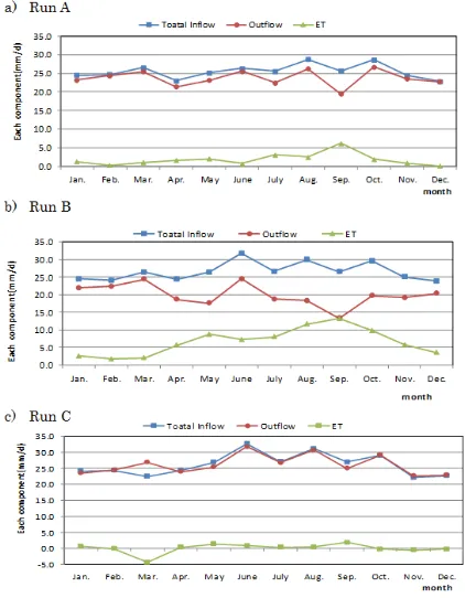
Figure 4 shows the variation of daily water balance (total inflow, daily precipitation and ET) of each run during the year of 2014. Figure 4-a is Run A, Figure 4-b is Run B, and Figure 4-c is Run C. As shown in the Figures 4-a, 4-b and 4-c, the majority of the total inflow were similar in the three runs during the experimental periods. In Figure 4, when there was high precipitation, total inflow and outflow remained fairly consistent in the three runs throughout the year of 2014.
In Figure 4-a, although it seems that there is no difference between the total inflow and outflow in Run A throughout the experimental periods, the outflow was slightly lower than the total inflow in the months between April and October. This may possibly be due to a small water loss by ET in Run A.
Figure 5. Monthly mean water balance of three runs for 2014: a) Run A, b) Run B and c) Run C
Figure 5 shows the monthly mean water balance of three runs for 2014. The ET was estimated on the basis of water budget method. Figure 5-a is the water balance of Run A, Figure 5-b is that of Run B, and Figure 5-c is that of Run C. In Figure 5-a, the ET rate of Run A gradually increased from April to September, and reached a small peak with an ET rate of 6mm/d in September. In Figure 5-b, starting in April, Run B rapidly reached a large peak with an ET rate of 14mm/d in
September and then decreased. The change in the ET rate and the outflow had a reversed relationship. In Figure 5-c, Run C had a very small ET throughout the year.
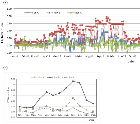
[image:6.595.94.516.85.627.2]varied from 0 to 0.4 during the period from April to October, which was the growing season for reeds. The ratio of ET to total inflow was around zero at the time of rainy weather and was within the range of 0.2 to 0.4 at the time of fine weather. That of Run B was within 0 to 0.2 during the period of the non-growing season for reeds and within the range of 0 to 0.8 during the period from the growing season for reeds. After May, the ratio of ET to total inflow was over 0.4 at the fine weather and showed to be near 0.8 in September, which meant that 80% of the total inflow was lost from HSF of Run B. That of Run C was within the range of 0 to 0.1 during the period of November to March and within the range of 0 to 0.4 during the period of April to October.
The daily variation of the ratio of ET to total inflow varied greatly depending on the presence or absence of precipitation, i.e, the greater the growth of the reed, the higher the ratio of ET to the total inflow.
As shown in Figure 6-b, the ratio of ET to total inflow of Run B which had a dense vegetation bed was within the
range of 0.24 to 0.56, with an average of 0.40 during the growing season from April to October, and within the range of 0.07 to 0.21, with an average of 0.12 during the non-growing season from November to March. On the other hand, that of Run A which had a poor vegetation bed was within the range of 0.04 to 0.26, with an average of 0.11 during the growing season, and within the range of 0.01 to 0.05, with an average of 0.03 during the non-growing season. That of Run C which was unplanted was within the range of 0.01 to 0.08, with an average 0.04 during the period from April to October, and from -0.03 to 0.02, with an average of -0.01 during the period of from November to March. The decrease of water loss by ET in Run B was higher compared to those of Run A and Run C during the non-growing season, and there was no or a little water loss by ET in Run A and Run C during the non-growing season. The ET in unplanted bed was very low throughout the year. The difference in growth of reeds greatly affected the ET rate in the HSF.
[image:7.595.67.524.320.725.2]Figure 7. Comparison of ET and PET: (a)Variation of monthly mean of PET and air temperature; (b)Comparison of monthly mean of ET and PET
3.4. Comparison of ET and PET
The PET was estimated on the basis of the Hamon equation. The Hamon equation was expressed as follow [19]:
PET=0.14D02Pi
PET: Potential evapotranspiration (mm/month), D0: Day time length (x/12hrs),
Pi: Saturated absolute humidity (mg/m3)
Figure 7 shows the comparison between ET and PET. Figure 7-a is the variation of the monthly mean of PET and the air temperature in 2014. The PET began higher with increasing the air temperature, reaching its peak in July, and the monthly air temperature reached its peak in August. The PET was strongly influenced by the air temperature, although the timing of the peak of the PET and the air temperature was different. Figure 7-b shows the comparison of the monthly average of PET and the monthly average of ET of the three runs. As shown in Figure 7-b, the ET of Run A and Run B began to increase with the air temperature rise and reached its peak in September. Although the pattern of the variation of the monthly mean ET of Run A and Run B looked similar, there was a large difference in the ET rate. On the other hand, the pattern of the variation of PET was quite different from those of Run A, Run B and Run C.
Figure 8 shows the annual precipitation, the annual ET rate of the three runs and the annual PET rate of 2014. The annual precipitation was 1343.5 mm, and the annual ET rates of Run A, Run B and Run C were 656.5, 2,434.3 and 22.2 mm respectively. The annual ET rate of Run B was 3.7 times that of Run A, and 110 times that of Run C. The growth difference in reeds provided a large difference in the annual ET rate. The annual ET rate of Run C was extremely small and the evaporation from the bed of Run C might be strongly suppressed. On the other hand, the annual PET rate was 751.5 mm, and was one-third of Run B. It was reported that the annual PET rate of Sendai, Japan was 689mm which was estimated by the Hamon equation and 697 mm by the Thornthwaite equation [20]. The 752 mm of PET rate in this study was close to those of previous studies. Thus, the PET which was estimated using the meteorological parameters
presented a significantly lower rate compared to the ET of Run B with a dense vegetation and did not reflect the actual ET. It was necessary to consider the site-specific factors such as the growth of plants in the evaluation of the water budget in the HSFs.
Figure 8. Annual precipitation, ET rate and PET Rate
4. Conclusions
The difference in the vegetation of reeds provided a large difference in ET, and the large ET in dense vegetation of reeds remarkably influenced the water budget. The ET increased with the growth of reeds and reached its peak in September. The ET in the dense vegetation bed was much higher than that of the poor vegetation bed in the non-growing season. The ET in the unplanted bed was very low throughout the year. Compared to the ET rate of the dense vegetation bed, the PET was much less. It was necessary to consider the site-specific factors such as the growth of plants in the evaluation of the water budget in the HSFs
REFERENCES
[1] Vymazal J. & Kropfelva L., 2008. Vegetation, Wastewater
1343.5
656.5
2434.3
22.2
751.6
0 500 1,000 1,500 2,000 2,500 3,000
precipitation Run A Run B RunC PET
mm/
Ye
[image:8.595.65.545.80.238.2] [image:8.595.316.546.337.475.2]Treatment in Constructed Wetlands with Horizontal Subsurface flow, Environmental Pollution 14, Springer, London, pp234-262.
[2] Matoh T., Matsushita, N. & Takahashi, E., 1988 Salt tolerance of the reed plant Phragmites Australis, Physiologia Plantarum, 72, pp. 8-14.
[3] Barr M. J. & Robinson H. D., 1994. Constructed wetlands for landfill leachate treatment, Waste Management & Research, 17(6), pp. 498-504.
[4] Mauchamp A. & Mesleard F., 2001 Salt tolerance Phragmites
australis populations from coastal Mediterranean marshes,
Aquatic Botany,70, pp. 39-52.
[5] Yano T., Kohama A., Arita K. & Enari K., 2010 Treatment of high salinity landfill-leachate using reed(Phragmites sp.),
Proceedings of 2nd Irish International Conference on
Constructed Wetlands for Wastewater Treatment and
Environmental Pollution Control, pp.5-12.
[6] Yano T., Okanuma M., Kumagai Y., Sato, K., Inoue -Kohama A. & Enari K., 2014. Growth Characteristic of Reeds (Phragmites australis) and Removal Performance in the Treatment of High Salinity Landfill-Leachates with Horizontal Subsurface Flow Constructed Wetlands,
14thInternational Conference Wetland Systems for Water
Pollution Control, USB Flash Drive, Shanghai, China.
[7] Yano T., Okanuma M., Kumagai Y., Sato K., Inoue-Kohama A. & Enari K., 2014. Effect of Salinity on in the treatment of high salinity landfill-leachate using HSF, J. Envron. Scie. & Eng., B3, pp. 142-150.
[8] Yano T., Yamada K., Nakayama M., Inoue-Kohama A., & Enari K., 2016. Evapotranspiration and Removal performance in the Treatment of High Salinity Landfill-Leachate using HSF,
J. Envron. Scie. & Eng., B5, pp. 440-450.
[9] Brix H. 1997 Macrophytes play a role in Constructed Wetlands?, Wat. Sci. Tecnol., 35(5), pp. 11-17.
[10]Tanner C. C. & Kadlec, R. H. 2003. Oxygen Flux Implications of Observed Nitrogen Removal Rates in Subsurface-Flow Treatment Wetlands, Water Sci. Technol., 48(5), pp. 191-198.
[11] Gangnon V., Chzarenc F., Comeau Y. & Brisson J., 2007 Influence of Macrophyte Species on Microbial Density in Constructed Wetlands, Water Sci. Technol., 56(3), pp. 248-254.
[12] Rozkosny M., Salec J. & Salec J.,2006. Water Balance of the Constructed Wetlands-A Study of the Macrophytes Evapotranspiration, Proceeding of 10th International
Conference on Wetland Systems for Pollution Control, Lisbon,
Portugal, pp.123-129.
[13] Brandon Lott R. & Hunt R. J., 2001. Estimating Evapotranspiration in Natural and Constructed Wetlands,
Wetlands, 21(4), pp. 614-628.
[14] El Hamouri, B., Nazih, J. & Lahjouj, J. 2007
Subsuraface-horazontal flow constructed wetland for sewage treatment under Moroccan climate conditions, Desalination, 215, pp.153-18.
[15] Headley T. R., Davidson L., Huett D. O. & Muller R., 2012 Evapotranspiration with Phragmites australis in sub-tropical Australia, Water Res., 46, pp.345-354.
[16] Bialowiec A., Wojnowska-Baryla I. & Agopsowicz M., 2007 The efficiency of evapotranspiration on landfill leachate in the soil-plant system with willow Silamix amygdarina L.,
Eco.eng., 30, pp. 356-361.
[17] Mulamoottil G., McBean E.A. & Rovers, F., editor., 2009 Constructed Wetlands for the Landfill Leachate, Leis Publishers, London, pp. 205-222.
[18] Kadlec R. M., Knight, R. L., Vymazal, J., Brix, H., Cooper, R. & Harberl, R., 2010. Constructed Wetlands for Pollution Control, Processes, Performance, Design and Operation,
Scientific and Technical Report No.8, IWA Publishing London,
UK, pp.41-54.
[19] Japan Society of Civil Engineers, 1985. Hydraulic Formula Handbook, Chapter 2, pp.144-145(in Japanese)
[20] Kobatake S., 1989 Estimation of Evapotranspiration Rate by Thronthwaite or Hamon equation, Annuals, Disas. Prev. Res.