Linear Minimum Variance Unbiased Estimation of Individual and Population slopes in the presence of Informative Right Censoring

Linear Minimum Variance Unbiased Estimation of

Individual and Population slopes in the presence of

Informative Right Censoring

Viswanathan.N

*

, Ravanan.R

**

*

Department of Statistics, Presidency College, Chennai 600005, India

**

Department of Statistics, Presidency College, Chennai 600005, India

Abstract- Estimation of individual and population slopes using Linear Minimum Variance Unbiased Estimation by Wu and Bailey (1988) is applied for incomplete longitudinal studies. In these studies the right censoring process is considered informative, in which the number of observations made for each subject is assumed to vary depending on the rate of change or slope of the individual response variable. This process of ‘missing not at random’ poses problems in the estimation of the slope parameters. The proposed method provides better estimates under different parametric models for the censoring distribution. The method’s performance is studied through a simulation study under Standard Normal and Uniform censoring distributions.

Index Terms- Cumulative distribution function, Empirical Bayes estimation, Standard Normal distribution, Probit function, Informative Right censoring, Simulation.

I. INTRODUCTION

haracterization of rate of change in the study variable over time is of primary interest in longitudinal studies, where repeated measurements of the study variables are taken on the subjects. The rate of change of these variables over time is one of the primary interests of the researchers, as it helps us track the individuals who are at risk or those who need immediate attention. The classical methods of estimation fail under the condition of ‘missing not at random’ or when the censoring distribution is dependent on the rate of change of the study variable of the individual subject. Longitudinal studies prolong for many years and entail dropouts due to deaths, migration and related factors. There are several proposed methodologies to accommodate incomplete data by Orchard and Woodbury (1982), Kleinbaum (1973) and Laird and Ware (1982). These methods assume patterns that accommodate dropouts that are independent of the study variable. In this paper, the pattern of missing data considered is related to the study variable.

The term 'informative right censoring' in the context of slope estimation refers to the situation where the censoring probability of each individual relates to his or her underlying rate of change (Wu and Bailey, 1988).They showed that under a linear random effect model the weighted least square estimate of slope can be severely biased if the right censoring process is informative, although it is most efficient if the censoring process is non-informative. In an effort to reduce the bias introduced by the presence of informative right censoring, Wu and Carroll

(1988) derived a Probit Pseudo-Maximum Likelihood Estimator (PPMLE) of the population rate of change under a linear random effect model where the right censoring process follows a probit function, both of initial value and of the slope of the individual subjects. Wu and Bailey (1989) adapted a conditional linear model approach and proposed a Linear Minimum Variance Unbiased (LMVUB) and Linear Minimum Mean Square Error (LMMSE) estimators of the population rate of change, which they showed were competitive with the PPMLE in their simulation study. The present study focuses the effectiveness of the LMVUB estimator under different censoring distributions, whose parameter depends on the rate of change of the individual study variable. LMVUB estimator is compared with the general Empirical Bayes estimator, Un-weighted and Weighted estimators. To measure its effectiveness, the study considers both the individual and population slopes. Simulation results are considered and inferences are made, with suggestions for the future research.

II. THEESTIMATIONPROCEDURE

The LMVUB estimator is derived from the general case of the Empirical Bayes estimation procedure. This model assumes that here are n subjects and that for each subject i (i = 1, 2 . . . , n) the following conditions hold:

(i)

b

i,ols

|



i

,

t

imi

~

N

(



i

,

V

i

)

(ii)



i

|



0

,



1

,

t

imi

~

N

(



0





1

*

t

imi

,

A

)

where

b

i,olsis the Ordinary Least Square (OLS) estimate of

the slope and

t

imi_{is the maximum time the i}th _{subject is followed} up.















i

m

j

i ij ols

i i

t

t

b

Var

V

1

2 2

,

)

(





, where

2





_{is a known constant}

and A= Var (



i_{) is also assumed to be known. Let}



t

i1

,

t

i2,

,

t

i3

,...,

t

im_i



_{denotes the vector of time points for the i}th

subject. It is assumed that the last measurement time,

t

imi _{is the}

censoring time. The marginal distribution of

b

i,ols is given

by

b

i,ols

|



0

,



1

,

t

imi

~

N

(



0





1

t

imi

,

A



V

i

)

_{, where}

1

0





and

are the parameters of the censoring distribution.

The posterior distribution of



i

given

b

i,ols is



1



)

,

(

~

,

,

,

|

i,ols 0 1 im i i i

i

b

t

i

N

V



B











,

where



i





1



B

i



b

i,ols



B

i





0





1

t

imi





, with V A

V B

i i i _

Let















1 0







and















n m m m

m

t

t

t

t

X

1 3

2

1

.

.

.

1

.

.

.

1

1

1

'

3 2 1 _.

Here the second row represents the individual censoring time of the subjects.

                                   A V A V A V A V D Let n 1 . . . 0 0 0 . . . . . . . . . . . . . . . . . . . . . 0 . . . 1 0 0 0 . . . 0 1 0 0 . . . 0 0 1 3 2 1















































n

B

B

B

B

B

and

.

.

.

0

0

0

.

.

.

.

.

.

.

.

.

.

.

.

.

.

.

.

.

.

.

.

.

0

.

.

.

0

0

0

.

.

.

0

0

0

.

.

.

0

0

3 2 1

The parameter



is estimated using the Weighted Least Square (WLS) method and is given by



X

'

DX



X

'

DB

ˆ

1





The Empirical Bayes estimate for the individual slope is given by



i



iols i



im_i



eb

i,

1

B

b

,

B

ˆ

0

ˆ

1

t

ˆ

_

_











; i =1, 2, 3, … ,n. Its matrix representation is given by



B



b

_ols

B

X



X

DX



X

DB

eb

1

'

'

ˆ

_

_

_

1



.

The corresponding estimator of the population slope is

given by







n i eb i eb pop

n

1 , ,

ˆ

1

ˆ

_



.

1



i

B

results in the LMVUB estimation.

The assumption of a conditional linear model is given by

i im i

i im t

im ols

i

t

t

b

_,

|





₀





₁





with

E

 



timi



0

_and

 

2

i im t i im t

Var







Then,

LMVUB

(



)





ˆ

0





ˆ

1

E

 

t

imi

If

B

ˆ

i



0

_{, it reduces to the Unweighted estimator and its}

population slope is given by







n i ols i uwt

b

n

1 ,

1

ˆ



. The weighted

individual slope estimator is



iwt



B

i



b

iols

B

i



wt

ˆ

1

ˆ

,

,







_with

the corresponding population slope estimator













     _n i i n i ols i i wt B b B 1 1 , 1 1 ˆ



.

III. SIMULATIONSTUDY

The simulation study is carried out to compare the performance of the four estimators: Empirical Bayes, LMVUB, Weighted and Unweighted Estimators. The study compares both individual and population slopes. Simulations are carried out for a setting similar to that already proposed and discussed in the literature by Wu and Baily (1988). R software is used to perform the simulation process. Parameters used in the simulation are similar to those of Wu and Baily, who obtained the estimates from a feasibility study for an anti-photolytic replacement therapy trial conducted by the Workshop on the Natural History of Piz Emphysema. The study variable in this trial is rate of decline in the FFV measurements. We generated 1000 data set, each containing 100 observations, according to the following specifications:

Measurement error standard deviation



=155; slope

censoring occurs only at the middle of each year, after the second measurement. The probability of right censoring or censoring

distribution during a specified time interval



0

,

t

j



_{, given the}

slope



i _{to be}







0j





1



i



_{, where}





.

_{is the cumulative}

probability distribution function of N (0, 1). The censoring

parameter for different time intervals are denoted by



0j, j =1, 2, 3. The simulations are carried out under 3 different conditions:

(1)



1_{= 0.00,}



01_{= - 1.41,}



02_{= - 0.71 and}



03_{= - 0.25; (2)}

1



_{= - 0.0113,}



01_{= - 3.04,}



02_{= - 2.04 and}



03_{= -}

1.38; and (3)



1_{= - 0.0138,}



01_{= - 3.26,}



02_{= -}

2.26 and



03_{= - 1.60; in the above scenario, the first set of}

parameters correspond to non-informative right censoring and the second and third conditions correspond to Informative right censoring. The simulation process is carried out with the following sequence.

(1)



i_{~ Normal (- 90,}

91

2_);

(2)

Pr

T

(



t

ij

|



i

)









0j





1



i



_{; and}

(3)

b

i,ols

|



i

,

t

1mi

~

_Normal





i

,

V

i



_{, where}















i

m

j

i ij ols

i i

t

t

b

Var

V

1

2 2

,

155

)

(

The criteria used to evaluate the performance are bias and two types of Mean Square Error MSE (a) and MSE (b) defined respectively as:

Bias (a) =











R

r r

R

1

ˆ

1

_

_

MSE (a) =











R

r r

R

1

2

ˆ

1

_

_

MSE (b) =







 



R

r n

i

ir ir

nR

1 1

2

,

ˆ

1

_

_

where R is the total number of replications, and n is the number of observations in each data set. MSE (a) measures the closeness of the estimator to the population slope and MSE (b) measures the closeness of the estimator to the individual slopes.

3.1 Random Generation of Censoring Distribution:

The censoring distribution, corresponding to the random

variable

m

i _{is generated using the}

assumption

Pr(

T



t

ij

|



i

)









0j





1



i



. Thus, the censoring distribution for each subject varies as



i _{varies from}

subject to subject. As



denote the cumulative distribution function of standard normal variate, the following procedure is

used to generate

m

i_values.

i. Four observations are made in three years amounting to

maximum (

m

i_{) = 12}

ii. Also it is assumed that right censoring occurs only at the middle of each year after the second measurement. This

implies

m

i_{takes values 2, 6, 10, 12.}

iii. For each of the three years the normal cumulative

probabilities with varying



0j j= 1, 2, 3 are calculated.

iv. The probability for

m

i_{= 2 is taken as the cumulative}

probability calculated for j=1. The probability for

i

m

=12 is taken as the difference between unity and the cumulative probability calculated for j= 3. The

probability for

m

i_{= 6 is taken as the difference between}

the cumulative probabilities for j = 2 and j = 1. The

probability for

m

i_{=10 is taken as the difference}

between the cumulative probabilities for j=3 and j=2. v. In case of Uniform cumulative distribution function the

upper and lower limits of the distribution are fixed by

Lower limit = Minimum (



i_)*



1_{+ Minimum (}



01_,



02_,



03₎

Upper limit = Maximum (



i_)*



1_{+ Maximum (}



01_,



02_,



03₎

The above procedure represents one of the ways of implementing





|

)

Pr(

T

t

_ij



_i







_0j





₁



_i



to generate random values for

m

i_.

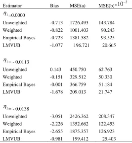
[image:4.612.172.439.85.373.2]

Table 3.1. Comparisons of bias and mean square error: Unweighted, Weighted, Empirical Bayes and LMVUB for Standard Normal distribution

the minimum MSE, followed by Weighted, Empirical Bayes and Unweighted estimators in that order. This trend is similar in both the population and individual slopes. Also to be noted is the magnitude of reduction in the MSE values. In case of Non-informative right censoring the MSE corresponding to the second best weighted estimator for population slope is nearly five times as that of the LMVUB estimator. In case of the individual slopes the MSE of Weighted estimator is 4.4 times as that of the LMVUB estimator.

In the presence of informative right censoring with



1



_-

0.0113, the LMVUB performs better compared to the other three estimators. The MSE has a similar pattern in this case, but with a reduced margin of the multiplicative factors. Considering the population slope the MSE of the second best weighted estimator is nearly 1.6 times as that of the corresponding LMVUB estimator. For the individual slopes the MSE of the weighted estimator is nearly 2.3 times as that of the corresponding LMVUB estimator.

With the scenario of informative right censoring with



1



- 0.0138, the MSE of the population slope for the second best

weighted estimator is nearly 6.8 times as that of the corresponding LMVUB estimator. For the corresponding individual slopes the MSE of the weighted estimator is nearly 4.8 times as that of the corresponding LMVUB estimator.

Comparing the bias in all the three scenarios, it is seen that the Empirical Bayes estimator performs better than LMVUB

estimator in cases with



1



_{0 and}



1



_{- 0.0113. In case of}



1



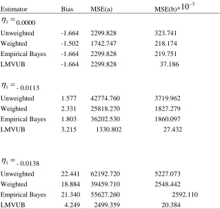
_{- 0.0138, the bias of the LMVUB estimator is the} minimum. In most of the estimators, it is seen that ‘over estimation’ of the parameters takes place.

Simulation results corresponding to the Uniform censoring distribution are provided in Table 3.2. In this case again, the dominance of LMVUB estimator can be seen in all but the case

for population slope with



1



_{0. By observing the MSE}

corresponding to population and individual slopes, the LMVUB estimator has the minimum, followed by Weighted, Empirical Bayes and Unweighted estimators in that order. This trend is similar in both the population slope and

Estimator Bias MSE(a) MSE(b)*

10

3

1



_=0.0000

Unweighted -0.713 1726.493 143.784

Weighted -0.822 1001.403 90.243

Empirical Bayes -0.723 1381.582 93.525

LMVUB -1.077 196.721 20.665

1



_{= - 0.0113}

Unweighted 0.143 450.750 62.763

Weighted -0.151 329.512 50.330

Empirical Bayes -0.001 366.759 51.184

LMVUB -1.678 209.013 21.747

1



_{= - 0.0138}

Unweighted -3.051 2426.362 208.347

Weighted -2.226 1352.662 122.453

Empirical Bayes -2.655 1875.357 126.923

[image:5.612.149.468.94.396.2]

Table 3.2. Comparisons of bias and mean square error: Unweighted, Weighted, Empirical Bayes and LMVUB for Uniform (0, 1) distribution

Estimator Bias MSE(a) MSE(b)*

10

3



1



_0.0000

Unweighted -1.664 2299.828 323.741

Weighted -1.502 1742.747 218.174

Empirical Bayes -1.664 2299.828 219.751

LMVUB -1.664 2299.828 37.186



1



_{- 0.0113}

Unweighted 1.577 42774.760 3719.962

Weighted 2.331 25818.270 1827.279

Empirical Bayes 1.803 36202.530 1860.097

LMVUB 3.215 1330.802 27.432



1



_{- 0.0138}

Unweighted 22.441 62192.720 5227.073

Weighted 18.884 39459.710 2548.442

Empirical Bayes 21.340 55627.260 2592.110

LMVUB 4.249 2499.359 20.384

as well in the individual slopes. Also, this pattern is similar to that of the one seen using the Standard Normal cumulative distribution.

In case of Non-informative right censoring with the population slope, the weighted estimator has the least MSE. The other three has marginally higher values. In case of the individual slopes the MSE of Weighted estimator is 5.9 times as that of the LMVUB estimator that has the minimum MSE.

In the presence of informative right censoring with



1



_-

0.0113, the LMVUB performs better compared to the other three estimators. Considering the population slope the MSE of the second best weighted estimator for the population slope is nearly 19.4 times as that of the corresponding LMVUB estimator. For the individual slopes, the MSE of the second best weighted estimator is nearly 66.6 times as that of the corresponding LMVUB estimator.

The scenario of informative right censoring with



1



_-

0.0138, the MSE of the population slope for the second best weighted estimator is nearly 15.8 times as that of the corresponding LMVUB estimator. For the corresponding individual slopes the MSE of the weighted estimator is nearly 125 times as that of the corresponding LMVUB estimator. Comparing the bias in all the three scenarios, it is seen that the Weighted estimator performs better in the non-informative situation, Unweighted estimator performing better in case of

informative right censoring with



1



_{- 0.0113 and the LMVUB}

performing better in the case of



1



_{- 0.0138. In the case}

of the Uniform censoring distribution for most of the estimators ‘over estimation’ of the parameter values takes place.

IV. DISCUSSION

Comparison with respect to the MSE under simulation study reveals the better performance of LMVUB estimator as an alternative to that of the Unweighted, Weighted and Empirical Bayes estimators in both the informative and Non-informative Right censoring scenarios. LMVUB estimator performs better in estimating both individual and population slopes. This advantage of LMVUB may be the result of the conditional linear modelling of the observed slopes with the censoring time that provides a better judgement of the rate of change in the response variable. As Little (1988) pointed out in the context of conditional linear models, the main idea of the Empirical Bayes estimator adapted here is to shrink not towards a common mean but towards a regression line where the mean is a linear function of the censoring time.

the scenarios. Wu and Bailey (1989) show that the conditional expectation of the slope, given the censoring time, is a monotonic function of the censoring time under the linear random effects model with probit censoring distribution.

Further theoretical work is necessary in the areas of testing the presence of informative right censoring. This requires estimating the standard errors for the population and individual slopes. The case when the variance parameters are unknown needs to be addressed separately. Subjects with one observation need to be accommodated, may be using other than slope construct, to fully utilize the available information.

REFERENCES

[1] Efron, B. and Morris, C (1975). ‘Data analysis using Stein’s estimator and its generalizations’, Journal of the American Statistical Association, 70, 31 1-319.

[2] Fearn, T (1975). ‘A Bayesian approach to growth curves’, Biometrika, 62, 89-100.

[3] Hui, S. L. and Berger, J. 0 (1983). ‘Empirical Bayes estimation of rates in longitudinal studies’, Journal of the American Statistical Association, 78, 753-760.

[4] Kleinbaum, D. G (1973). ‘A generalization of the growth curve model which allows missing data’, Journal of Multivariate Analysis, 3, 117-124.

[5] Laird, N. M. and Ware, J. H (1982). ‘Random-effects models for longitudinal data’, Biometrics, 38, 963-974.

[6] Morris, C. N (1983). ‘Parametric empirical Bayes inference: Theory and applications’, Journal of the American Statistical Association, 78, 47-55. [7] Orchard, T. and Woodbury, M. A (1972). ‘A missing information principle:

Theory and applications’, Proceedings of the 6th Berkeley Symposium on Methods in Statistics and Probability, 1, 697-715.

[8] Searle, S. R (1971). Linear Models, Wiley, New York.

[9] Wu, M. C. and Bailey, K (1988). ‘Analyzing changes in the presence of informative right censoring caused by Death and withdrawal’, Statistics in Medicine, 7, 337-346.

[10] Wu, M. C. and Bailey, K (1989). ‘Estimation and comparison of changes in the presence of informative right Censoring: Conditional linear model’, Biometrics, 45, 939-955.

[11] Wu, M. C. and Carroll, R. J (1988). ‘Estimation and comparison of changes in the presence of informative right Censoring by modeling the censoring process’, Biometrics, 44, 175-188.

AUTHORS

First Author – Viswanathan.N, M.Sc., Assistant Professor,

Department of Statistics, Presidency College, Chennai, [email protected]

Second Author – Dr. R. Ravanan, M.Sc., M.Phil., Ph.D.,

Associate Professor & Head, Department of Statistics,