M E T H O D O L O G Y
Open Access
A multi-criteria spatial deprivation index to support
health inequality analyses
Pablo Cabrera-Barona
*, Thomas Murphy, Stefan Kienberger and Thomas Blaschke
Abstract
Background:Deprivation indices are useful measures to analyze health inequalities. There are several methods to construct these indices, however, few studies have used Geographic Information Systems (GIS) and Multi-Criteria methods to construct a deprivation index. Therefore, this study applies Multi-Criteria Evaluation to calculate weights for the indicators that make up the deprivation index and a GIS-based fuzzy approach to create different scenarios of this index is also implemented.
Methods:The Analytical Hierarchy Process (AHP) is used to obtain the weights for the indicators of the index. The Ordered Weighted Averaging (OWA) method using linguistic quantifiers is applied in order to create different deprivation scenarios. Geographically Weighted Regression (GWR) and a Moran’s I analysis are employed to explore spatial relationships between the different deprivation measures and two health factors: the distance to health services and the percentage of people that have never had a live birth. This last indicator was considered as the dependent variable in the GWR. The case study is Quito City, in Ecuador.
Results:The AHP-based deprivation index show medium and high levels of deprivation (0,511 to 1,000) in specific zones of the study area, even though most of the study area has low values of deprivation. OWA results show deprivation scenarios that can be evaluated considering the different attitudes of decision makers. GWR results indicate that the deprivation index and its OWA scenarios can be considered as local estimators for health related phenomena. Moran’s I calculations demonstrate that several deprivation scenarios, in combination with the‘distance to health services’factor, could be explanatory variables to predict the percentage of people that have never had a live birth.
Conclusions:The AHP-based deprivation index and the OWA deprivation scenarios developed in this study are
Multi-Criteria instruments that can support the identification of highly deprived zones and can support health inequalities analysis in combination with different health factors. The methodology described in this study can be applied in other regions of the world to develop spatial deprivation indices based on Multi-Criteria analysis.
Keywords:Deprivation, Analytical Hierarchy Process (AHP), Ordered Weighted Averaging (OWA), Geographically Weighted Regression (GWR), Health
Resumen
Antecedentes:Índices de privación son medidas útiles para analizar inequidades en salud. Existen varios métodos para construir estos índices, sin embargo pocos estudios han usado Sistemas de Información Geográfica (SIG) y métodos Multi-Criterio para esta construcción. Este estudio aplica Evaluación Multi-Criterio para calcular los pesos de los indicadores del índice de privación, y también un enfoque SIG de lógica difusa para crear distintos escenarios de este índice.
(Continued on next page)
* Correspondence:pablo.cabrera-barona@stud.sbg.ac.at
Interfaculty Department of Geoinformatics - Z_GIS, University of Salzburg, Schillerstraße 30, 5020 Salzburg, Austria
(Continued from previous page)
Métodos:El Proceso Analítico Jerárquico (AHP) es usado para obtener los pesos de los indicadores del índice. La Sumatoria Lineal Ordenada Ponderada (OWA) que usa cuantificadores lingüísticos es aplicada para crear diferentes escenarios de privación. La Regresión Ponderada Geográficamente (GWR) y el índice Moran’s I son empleados para explorar relaciones espaciales del índice de privación y sus escenarios, con dos factores relacionados a salud: distancia a servicios de salud y porcentaje de personas que nunca han tenido un nacido vivo. Este último indicador fue considerado como la variable dependiente de la GWR. El caso de estudio es la Ciudad de Quito, en Ecuador.
Resultados:El índice basado en el método AHP muestra media y alta privación (0,511 a 1,000) en zonas específicas del área de estudio, no obstante, la mayoría del área de estudio tiene bajos niveles de privación. Los resultados de OWA muestran escenarios de privación que pueden ser evaluados considerando diferentes actitudes de los tomadores de decisión. Los resultados de GWR indican que el índice de privación y sus escenarios OWA pueden ser considerados como estimadores locales de fenómenos relacionados a la salud. Los cálculos de Moran’s I demuestran que varios escenarios de privación, en combinación con el factor de‘distancia a servicios de salud’, podrían ser variables explicativas del porcentaje de personas que nunca han tenido un nacido vivo.
Conclusiones:El índice basado en el método AHP y los escenarios OWA de privación son instrumentos de análisis Multi-Criterio que pueden apoyar a la identificación de zonas con pobreza, y en combinación con otros factores de salud, pueden apoyar al análisis de inequidades en salud. La metodología descrita puede ser aplicada en otras regiones del mundo para desarrollar índices de privación basados en análisis Multi-Criterio.
Palabras clave:Privación, Proceso Analítico Jerárquico, Sumatoria Lineal Ordenada Ponderada, Regresión Ponderada Geográficamente, Salud
Background
Approaches to developing deprivation indices are diverse [1-4], and area-based deprivation indices have been proven to be useful in identifying patterns of inequalities in health outcomes [1-11]. Deprivation can be defined as any disad-vantage of an individual or human group, related to the community or society to which the individual or human group belongs, and these disadvantages can be of social or material nature [4,5]. Social deprivation can be linked to concepts of social fragmentation [11], and material deprivation can be related to the concept of poverty in terms of the lack of basic goods. These two kinds of deprivation are closely linked to public health and wellbeing [12]. Measuring deprivation requires the identification of two main issues: which indicators to be used to construct a deprivation index, and how to combine these indicators. The criteria for choosing the different indicators that com-pose deprivation indices can vary. In general, they depend on the availability of information in census and the object-ive of the study [2-4,8,9]. There are referential studies on constructing multiple deprivation indices, such as the Townsend Deprivation Index, which uses four indicators of material and social deprivation [4]; the Under Privileged Area score, also known as the Jarman Deprivation score, which considers eight deprivation indicators, and has been used to determine remuneration for physicians in United Kingdom [13,14]. Another known measure is the Carstairs deprivation index [15], which is very similar to the Town-send index but is a Scottish reality-based index. Common indicators for these three indices are overcrowding and
unemployment. Townsend and Carstairs indices also in-clude a very specific variable available in the British Census, namely the indicator of“Non car ownership”. More recent efforts have used other kinds of indicators from different domains, including health, housing and vulnerability of the population, for the construction of deprivation indices [1-3,6-9]. However, the most common deprivation domains that can support studies of health are related to occupation, education and household conditions, including overcrowd-ing [3]. Once the indicators for a deprivation index are chosen, the next important step is to define how they are going to be combined. Deprivation indicators can be com-bined using (i) simple additive techniques, using (ii) weights for each indicator, or using (iii) multivariate techniques [16]. The first technique just adds the deprivation indicators [4,16], the second technique can include expert-based weights [17], and the third technique commonly uses indi-cators weights created using statistical analysis such as the Principal Component Analysis [2,18].
Deprivation indices are constructed by integrating in-dicators generally extracted from census areas data [18,19]. In many parts of the world where census data are available, such indices can be geo-referenced using GIS. Subsequently, such geo-referenced data allow fur-ther spatial analyses, such as investigating spatial corre-lations [20], performing accessibility analysis [21], analyzing geographical patterns [22] or studying multiple scale evaluations [10] of deprivation measures.
little discussion so far about the spatial perspectives of these indices [10,17,22]. There is also not much docu-mented experience - at least not through systematic com-parisons of different scenarios - on how to construct these indices spatially.
Based on this background, this paper shows the de-velopment of a deprivation index using techniques from Multi-Criteria decision making [8,17,23] and GIS-based fuzzy methods [17,24]. This methodology will show how an Analytical Hierarchy Process (AHP) is applied to obtain the weights for the different indi-cators that make up the deprivation index. AHP is a Multi-Criteria evaluation method that takes informa-tion from experts’judgments [23]. We then apply Or-dered Weighted Averaging (OWA) in order to create different deprivation scenarios [17]. The indicators used to construct our spatial deprivation index follow a rights-based approach [25,26], and are extracted from the 2010 Ecuadorian Population and Housing Census. This rights-based approach prioritizes latent prob-lems in Latin America, where basic needs probprob-lems (for example, not having sewerage systems) are more common than, for example, in European countries. The indicators used represent education, health, employment and housing conditions in census blocks of our study area, Quito City, Ecuador. This area has a total of 4034 census blocks, and the census block is considered the smallest area from which census information could be extracted.
A spatial explorative analysis using Geographically Weighted Regression (GWR) and Moran’s I is applied to the deprivation index and its scenarios to evaluate how they are spatially related to the following health factors: distance to health services, and the percentage of people that have never had a live birth. The distance to health services is considered a variable of health accessibility that could be considered in relation to deprivation mea-sures in order to identify its effects on health [21]. The health factor of the percentage of people that have never had a live birth is related to a Population Census variable called “number of people that have never had a live birth”. This indicator can represent health inequalities: when a woman’s child is not born alive, this could be considered to be a consequence of a health condition, such as reproductive or maternal health problem [27]. This indicator can be calculated using information avail-able in the 2010 Ecuadorian Population and Housing Census, and therefore could be considered a useful health-related indicator that can be analyzed together with deprivation indices to be obtained from future Cen-sus data. This variable is obtained from women’s answers about how many live births they have had. At the time of a child’s birth, he or she is considered to be a “live birth”if he or she shows vital life signals such as breath-ing and movement.
Methods
Study area and materials
The case study is the urban area of the Metropolitan District of Quito, Ecuador (Figure 1). This area is known as Quito City, and is home to more than 1.5 million people distributed in 34 urban districts (Parishes) [28]. This urban area has a narrow shape due its limits with the Pichincha Volcano in the west and the Valleys of Tumbaco and Los Chillos to the east. Over 80% of inhabitants are mestizos (mixed-ethnicity people) [28] but the city is also inhabited by minorities such as indigenous people, black people and white people. Historically, the south of Quito City was home to blue collar workers, as well as being the area where several factories and companies have settled [29]. In contrast, the north was inhabited by wealthier people. However, due the influx of migrants from other areas of the country and the population growth [30], there is not a single rule to locate different socio-economic groups in the city today, and we can find very poor neighborhoods in the north, and very new and up-market condominiums in the south.
The information to construct the deprivation index was derived from the 2010 Ecuadorian Population and Housing Census [28]. The advantages of using Popula-tion and Housing Census informaPopula-tion to construct indi-ces are that census data are commonly open acindi-cess, and follow a standardization that allows a comparison of in-formation between different places and time. A geo-coded shape file of census blocks was also used in order to link the 2010 Census data to the 4034 census areas that make up the study area.
For the calculation of the distance to health services, a data set of the geo-referenced health services in Quito City was used. This data set was provided by Ecuador’s Ministry of Health.
Multi-Criteria Evaluation
A Multi-Criteria Evaluation (MCE) includes knowledge derived from different resources that can be integrated with GIS methods in order to support different kinds of analyses [23]. MCE combines information obtained from different criteria to produce an evaluation index [31] and a weight is allocated to each criterion, to represent the im-portance of the criterion. In this study, the Analytical Hierarchy Process (AHP) was applied. AHP is a MCE method developed by Saaty [32] that offers practical sup-port for decision making and a straightforward way to ob-tain weights from criteria [23]. MCE methods, including AHP, also have the capacity to be integrated into GIS-based environments [23,24,33-36] and these GIS-GIS-based MCE approaches have been widely and successfully ap-plied in environmental analysis [23,24,31,33,35,37].
criteria are factors or variables that are considered to de-termine deprivation. A rights-based approach was used to choose the factors that make up the deprivation index [25,26], taking into account the framework ofBuen Vivir (Good Living), that is based on human rights and nature rights. TheBuen Vivirconcept considers that in order to achieve a better quality of life, including time for leisure and harmony with nature, basic needs should first be satisfied [26].Buen Vivircannot be achieved if people do not have access to services that ensure their wellbeing and allow them to develop capabilities that create equal opportunities for everyone [26]. To have a good educa-tion, health, and to live in conditions of dignity, encour-ages actions that allow people to construct cohesive societies of Good Living. Human rights are universal. Therefore, the Buen Vivir concept can be applied in other countries, and it is not a concept which focuses only on Ecuador.
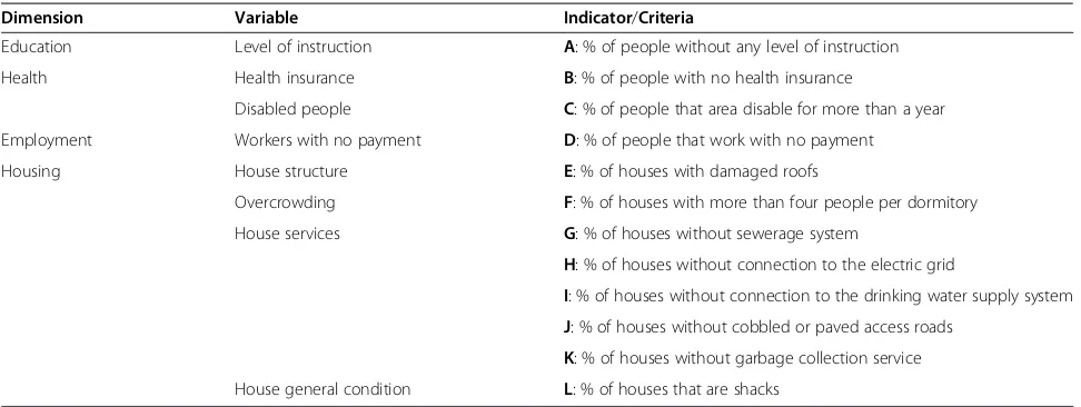
Table 1 shows the different indicators considered for the construction of the deprivation index. Each indicator is considered as a criterion for the AHP. The chosen indica-tors fulfill the following requirements: i) to consider a hu-man rights-based approach, ii) to be related to health and to have an affinity with material or social dimensions of deprivation [2,3,11,18,21] and iii) to be able to be repre-sented at the census block level [2]. The chosen indicators belong to the dimensions of education, health, employ-ment and housing conditions.
Variances Inflation Factors (VIF) were calculated for
all indicators used in order to identify
multi-colinearities. VIF shows how much the variance of an es-timated regression coefficient is increased as a result of the colinearities between two variables. All VIF obtained were less than 5, which means all selected indicators can be used for the construction of the index.
The key step in any AHP is the creation of a pairwise comparison matrix to compute weights for each criter-ion while reducing the complexity of the phenomenon in question, because only two criteria are compared at one time [38]. For the comparison of the resulting pair-wise matrix, a unified scale is used. The grade of import-ance of each indicator is evaluated in relation to all other indicators. The importance scale ranges from 1 to 9, whereby 1 means equal importance, 3 means moder-ate importance, 5 means strong or essential importance, 7 represents very strong importance and 9 indicates ex-treme importance. Values of 2, 4, 6 and 8 can also be used and are considered as intermediate values.
In order to obtain the references for the grades of im-portance, 32 experts’judgments were taken into consider-ation. The consulted experts are members of public and private Ecuadorean Institutions and work in the fields of Medicine, Geography and Territorial Planning, Environ-mental Sciences, and Social Sciences. They were consulted via an online questionnaire in September, 2014. The results of the pairwise comparison matrix are shown in Table 2, and the importance scores show that, according to the ex-perts, the chosen indicators are of equal or very similar im-portance: for example, indicator B (% of people with no health insurance) is of the same importance as indicator A (% of people without any level of instruction), and indicator D (% of people that work with no payment) is of moder-ately greater importance than indicator C (% of people that are disabled for more than a year). The pairwise compari-son matrix is reciprocal, consequently it is only necessary
to fill in one diagonal half of the matrix. After assigning the different levels of importance in the pairwise comparison matrix, a normalized matrix (N) is obtained as described below [39]:
N¼ Xaij
aij
The normalized value for each cell ofNis obtained by calculating the ratio of each importance valueαij of the pairwise comparison matrix and the values sum of each column of this matrix.
Afterwards, all the row values of the normalized matrix are added, and then the sum is divided by the number of the indicators used to construct the deprivation index. The result of this operation is a vector that contains the weights for each indicator (criterion), the eigenvector.
One of the potentials of AHP is that one can evaluate the consistency of the experts’judgments, by calculating a consistency ratio (CR) that indicates the likelihood that the pairwise comparison matrix judgments were gener-ated randomly [32]:
CR¼CIRI
WereCIis the consistency index andRIis the random index.CIis calculated using the equation:
CI¼λmaxn−−n 1
Wheren represents the number of criteria and λmax is obtained as follows: a second vector is obtained by multi-plying the eigenvector and the pairwise comparison matrix. Then a third vector is obtained by dividing the values of the second vector by the values of the eigenvector.λmaxis the average of all the components of this final vector [39]. Table 1 Criteria to construct the deprivation index
Dimension Variable Indicator/Criteria
Education Level of instruction A: % of people without any level of instruction
Health Health insurance B: % of people with no health insurance
Disabled people C: % of people that area disable for more than a year
Employment Workers with no payment D: % of people that work with no payment
Housing House structure E: % of houses with damaged roofs
Overcrowding F: % of houses with more than four people per dormitory
House services G: % of houses without sewerage system
H: % of houses without connection to the electric grid
I: % of houses without connection to the drinking water supply system
J: % of houses without cobbled or paved access roads
K: % of houses without garbage collection service
RI represents the consistency index of a random pair-wise comparison matrix [38] and the values that this index can take depends of the number of criteria used [39]. Table 3 shows different values for the RI. In this study, we worked with twelve criteria or indicators, therefore theRIvalue used is 1,48.
The CR obtained was 0,0019, a value lees than 0,10. This value means that the pairwise comparison matrix is satisfactory [39], which is to say that there is a reason-able level of consistency in the experts’ judgments [38,40]. The weights obtained for each indicator and the
CRare also showed in Table 2.
A first representation of the deprivation index was cal-culated based on the AHP weights by adding the
deprivation weighted indicators. Linear min-max
normalization was applied to this deprivation index. Values closer to 1 represent higher deprivation. We call the result of this calculation the AHP-based deprivation index.
Ordered Weighted Averaging (OWA)
The Ordered Weighted Averaging (OWA) provides an extension of the Boolean and weighted aggregation oper-ations [39,41]. It ranks the criteria in a MCE and ad-dresses the uncertainty from criteria interaction [24]. OWA works not only with criteria weights (wj. j = 1,2,3, …, n) but principally with order weights (vj. j = 1,2,3,…,
n). Criteria weights are assigned to each criterion and in-dicate the level of importance of each criterion [42]. We applied AHP to calculate criteria weights. On the other hand, order weights depend on the ranking of each
criterion rather than on its attributes. Order weights are assigned differentially in each location, depending on the respective criterion rank order [43]:
For example, if v1, v2 and v3 are order weights that
have to be applied to the AHP-based weighted criteria X, Y and Z, for instance, if at one location the rank order is YXZ and in another location it is ZYX, the order weights are assigned as v1* Y +v2* X +v3* Z and v1* Z
+v2* Y +v3* X, respectively.
The OWA operator is defined as follows [44-46]:
OWAi¼
Xn
j¼1
ujvj
Xn
j¼1ujvj
0 @
1 Azij
Where uj is the criterion weight reordered according to each criterion attribute value, vj is the order weight and Zijis the sequence obtained by reordering the attri-bute values. When using different order weights, differ-ent results can be produced. From a GIS-based perspective, therefore, using different Boolean operations such as union (OR) and intersection (AND), or weighted linear combination [43-46] will result in different spatial patterns.
The key issue in OWA is to obtain the order weights. We used linguistic quantifies to support the production of the order weights [42,44]. Linguistic quantifiers allow to translate natural language into mathematical formula-tions [42]: if we consider thatQis a linguistic quantifier, it can be represented as a fuzzy set over the interval 0 to 1, and if we consider that pis a value belonging to this Table 2 Results of the AHP method
Indicator (Criteria) A B C D E F G H I J K L Weightswj
A 1 0,0757
B 1 1 0,0757
C 1/2 1/2 1 0,0408
D 2 2 3 1 0,1410
E 1 1 2 1/2 1 0,0757
F 1 1 2 1/2 1 1 0,0757
G 2 2 3 1 2 2 1 0,1410
H 1 1 2 1/2 1 1 1/2 1 0,0757
I 2 2 3 1 2 2 1 2 1 0,1410
J 1/2 1/2 1 1/3 1/2 1/2 1/3 1/2 1/3 1 0,0408
K 1 1 2 1/2 1 1 1/2 1 1/2 2 1 0,0757
L 1/2 1/2 1 1/3 1/2 1/2 1/3 1/2 1/3 1 1/2 1 0,0408
Consistency ratio (CR): 0,0019.
Table 3 Random indices
n 1 2 3 4 5 6 7 8 9 10 11 12 13 14 15
interval,Q(p) represents the compatibility ofpwith the concept referred to by the quantifierQ[42,44] and is de-noted by:
Q pð Þ ¼p∝; ∝>0
Where the parameter ∝ changes depending on which linguistic quantifier it belongs to, and can vary from,“at least one”to“all”quantifiers [38,42,44].
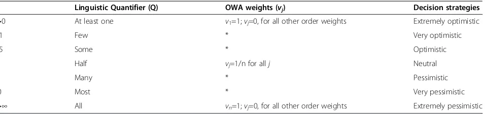
We used regular increasing monotone (RIM) quanti-fiers that produce order weights related to measures of ORness and tradeoff [42,44,46,47]. Table 4 shows the dif-ferent values that the parameter∝can take.
In the OWA procedure, it is very important to evalu-ate the decision strevalu-ategies. These strevalu-ategies range be-tween extremely optimistic and extremely pessimistic. These strategies are to be interpreted according to the following logic: in the extremely optimistic strategy, the decision maker’s attitude leads to weighting the highest possible outcome value (for this study the outcome value is the value of deprivation). From a probabilistic per-spective, an extremely optimistic strategy is a situation in which a probability of 1, the highest probability, is assigned to the highest value at each location [45]. In other words, the highest ordered weight is assigned to the highest value at each location. The linguistic quanti-fier for the extremely optimistic strategy is “At least one”, and this linguistic quantifier is equivalent to the logic OR (union) [44], meaning that something is true if at least one logic operand is true.
The other extreme is the extremely pessimistic strat-egy, where the decision maker’s attitude leads to weight-ing the lowest possible outcome value. From a probabilistic perspective, in this strategy, the probability of 1 is assigned to the lowest value at each location [45]. The linguistic quantifier for the extremely pessimistic strategy is “All”, and this linguistic quantifier is equiva-lent to the logic AND (intersection) [44], meaning that something is true if all logic operands are true.
The neutral decision strategy represents a full-tradeoff between criteria, where equal order weights are applied to all possible values at each location. When increasing
the degree of optimism from the neutral strategy, greater order weights are assigned to the higher criterion values and smaller weights to the lower criterion values.
In this study, we used the following GIS-based MCE equation to calculate order weights for OWA [44]:
vj¼
Xj
k¼1
uk
!∝
− X
j−1
k¼1
uk
!∝
Finally, the linguistic quantifier-based OWA is defined as follows [44]:
OWAi¼
Xn
j¼1
Xj
k¼1
uk
!∝
− X
j−1
k¼1
uk
!∝!
zij
Table 5 provides an illustration of how to compute OWAifor the case of∝= 2 (for the RIM equals“Many”)
considering four hypothetic variables, each one with its respective weight.
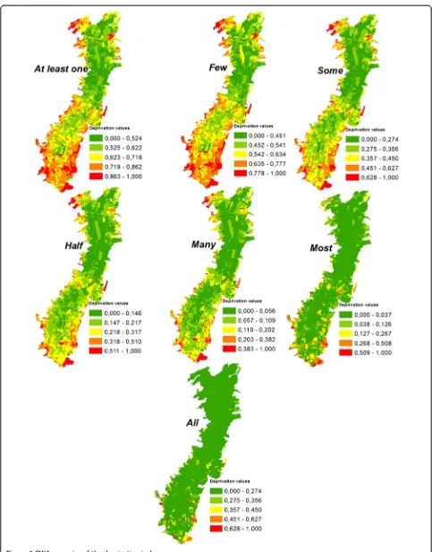
The process described in our illustration was applied to all the 4034 census blocks of our study area, for all the 12 chosen indicators, for each one of the seven quantifiers: At least one (Extremely optimistic), Few (Very optimistic), Some (Optimistic), Half (Neutral), Many (Pessimistic), Most (Very pessimistic) and All (Ex-tremely pessimistic).
In order to process this large amount of information, we developed a tool to compute the Ordered Weighted Aver-age with fuzzy quantifiers based on the method presented by Malczewski [44]. The tool is implemented as a Python toolbox in ArcGIS software (ESRI, Redlands, USA). Python is an open-source programming language that can be used in a wide variety of software application domains. Our Python toolbox uses a Python package for scientific com-puting called NumPy. During computation, NumPy is instructed to apply the appropriate mathematical functions to compute the Ordered Weighted Average. Using the tool requires entering a feature layer with the criteria as attri-butes. The Graphical User Interface of the tool is displayed in Figure 2. To use the tool, the user must browse to the feature layer, then select the criteria from the drop-down list and enter the weight for each criterion. After the
Table 4 Properties of Regular Increasing Monotone (RIM) quantifiers
∝ Linguistic Quantifier (Q) OWA weights (vj) Decision strategies
→0 At least one v1=1;vj=0, for all other order weights Extremely optimistic
0,1 Few * Very optimistic
0,5 Some * Optimistic
1 Half vj=1/n for allj Neutral
2 Many * Pessimistic
10 Most * Very pessimistic
→∞ All vn=1;vj=0, for all other order weights Extremely pessimistic
criteria and the weights are entered, the fuzzy quantifier must be selected from a dropdown list. This list has seven decision strategies: At least one (Extremely optimistic), Few (Very optimistic), Some (Optimistic), Half (Neutral), Many (Pessimistic), Most (Very pessimistic) and All (Ex-tremely pessimistic). After the decision strategy is selected, the location for the output feature layer must be entered. The output feature layer is a copy of the input feature layer with the OWA values attached as an attribute.
We applied the tool to compute the OWA for the 4034 census blocks. While the tool is running, the lin-guistic quantifier selected is translated to a numeric par-ameter ∝ where the values assigned are: 0,001 for At least one, 0,1 for Few, 0,2 for Some, 1 for Half, 2 for Many, 10 for Most and 1000 for All [44]. Using the tool, the OWA was computed for all seven decision strat-egies, yielding seven scenarios for the deprivation index. These seven scenarios were normalized on a scale from 0 to 1 using linear min-max normalization.
Spatial relationships between the different deprivation measures and health factors
Two health indicators were chosen to evaluate the relation of the OWA deprivation scenarios and the AHP-based
deprivation index with health: the distance of each census block to the nearest health service and the percentage of people in each census block that have never had a live birth. These two health indicators represent two different direct measures of the health dimension: a spatial measure of distances and a social measure of a health outcome. For the indicator of distance to health services, first, the cen-troids for each of the 4034 census blocks were calculated. Sizes of the census blocks differed all over the study area (sizes from around 3200 square meters to sizes of more than 400 000 square meters), therefore, centroids are a good representation of each census block location. Then, 128 health services were identified in the study area and the distances from each census block centroid to the near-est health service were calculated.
The indicator of percentage of people that have never had a live birth was calculated for each census block, using information available in the 2010 Ecuadorian Population and Housing Census: the“number of people that have never had a live birth” and the population of each census block.
Geographically Weighted Regression (GWR) was applied considering the measures of deprivation and distance to health services as the explanatory variables. The indicator Table 5 Illustration of OWA calculation for four criteria values, for the linguistic quantifier 2
j Criterion
values
Criterion weightswj
Ordered criterion valueszij
Ordered criterion weightsuij
Xj
k¼1
uk
!∝
vj vj*zij
1 0,20 0,30 0,80 0,35 (0,35)2= 0,1225 (0,1225 - 0) = 0,1225 0,098
2 0,80 0,35 0,50 0,10 (0,45)2= 0,2025 (0,2025 -0,1225) = 0,08 0,04
3 0,50 0,10 0,30 0,25 (0,70)2= 0,49 (0,49-0,2025) = 0,2875 0,08625
4 0,30 0,25 0,20 0,30 (1)2= 1 (1–0,49) = 0,51 0,102
∑ 1 1 1 OWAi=0,33
of percentage of people that have never had a live birth was considered as the dependent variable. A different GWR was made for each OWA scenario of deprivation and for the AHP-based deprivation index. GWR is an exten-sion of the standard regresexten-sion techniques that allows parameters βk to vary spatially. GWR evaluates the variations of the regression model relationships across space and, contrary to simple regressions, GWR allows local parameter estimates [48-50]. The GWR model can be written as:
Y sð Þ ¼i β0ð Þ þs
XM
k¼1
βkð ÞsXkð Þ þsi εð Þsi
This equations means that at every locations, all coeffi-cientsβkneed to be estimated, andε(si) is a random error with a mean of zero and a constant variance [50].
The estimations of coefficients βk require the weight-ing of all observations, and the weights are a function of the distance between the locationsand the observations around this location [49]. The function to calculate the weights is the kernel function:
wij¼exp h
α
ij b
Where wij is the weight of location sj that is used to estimate a parameterβkat the location si, and hαij is the distance between observationssjandsi[50].
The aim of applying GWR in this study is to explore how the AHP-based deprivation index and its OWA scenarios relate to health factors by determining the spatial correlations of these relationships. The GWR technique is complemented with the application of the Global Moran’s I.
Moran’s I is an index to measure spatial autocorrel-ation by comparing the value of a variable of one loca-tion with the value of this variable at all other locations [51]. Moran’s I is defined by the following equation:
I¼n
Xn
i¼1
Xn
j¼1wijðxi−xÞ xj−x
X
i
X
j≠iwij
Xn
i¼1ðxi−xÞ 2
Where n is the number of spatial units to be taken into account, x is a value of a unit, x is the mean of all values across all n units, and wij is the spatial
weight matrix that is a function of the distance that de-scribes the neighborhood of spatial units. A positive Moran’s I indicates the existence of clusters of similar values, while a negative Moran’s I indicates clusters of dissimilar values. Moran’s I closer to 0 indicates weak autocorrelation [52].
Results and Discussion
Deprivation index and its OWA scenarios
The AHP-based deprivation Index results (Figure 3) dis-play the presence of medium and high levels of deprivation (0,511 to 1,000) in specific zones of the study area, even though most of Quito City has low values of deprivation. Higher levels of deprivation appear at the edges of the study area, and represent relatively recently settled neigh-borhoods created by socio-economically more deprived people. On the other hand, lower deprivation levels (0,000 to 0,146) are commonly present on the northern side of the City, a part of Quito generally inhabited by people with better socio-economic conditions. Moderately deprived areas are located in the south, a very industrial and com-mercial area, traditionally inhabited by blue collar workers. These results coincide with what was explained in the study area description and confirm the consistency (Consistency ratio CR: 0,0019) of the AHP weights derived from the experts’judgments. The AHP-based deprivation Index has been shown to be very useful to evaluating levels of socio-economic deprivation considering our human rights-based approach: deprivation caused by unsatisfied needs due to a lack of basic services and capabilities related to human rights. For example, people with lower levels of education and health that live in unworthy households with limited or no access to basic services are considered to have high levels of deprivation in many socio-economic dimensions.
values and smaller weights are assigned to the higher cri-terion values.
The deprivation scenario with the linguistic quantifier “All”(logic AND) is considered the“worst-case scenario” [44] and in the case of our study, the worst-case scenario means that no action needs to be taken regarding the socio-economic deprivation in almost the entire Quito City territory. Nevertheless, this scenario could be useful to detect the most deprived areas, and can discern areas where taking immediate action is required to reduce socio-economic deprivation. On the other hand, the deprivation scenario with the linguistic quantifier “At least one” (logic OR), representing extreme optimism, shows larger deprivation areas. With this strategy, a lar-ger number of deprivation areas should be considered for socio-economic recuperation, but this may not be feasible for decision makers due to time- and financial
constraints. The “Half” scenario means that if the deci-sion makers’ risk-taking is neutral, only the AHP deprivation index constructed based on the experts’ judgments can be considered. The “Few” and “Some” scenarios could support decision making that identifies areas where an extensive social-improvement program could work for most of the city, while the scenarios “Many” and “Most” could support decision making that focuses on taking action in highly socio-economically deprived areas without excessive financial/time investment.
Spatial relationships between the different deprivation measures and health factors
kernel is determined using the Akaike Information Criter-ion (AIC). The AIC is a relative measure of a statistical model quality that takes into account the statistical good-ness of fit and the tradeoff of the parameters used in the model. There is no range of values for this measure and the best model is considered to be the one with the lowest AIC value. The GWR models that have the best goodness of fit are the “AHP-based” model and the “Half” model. Other models with low AIC values are the “Some” and “Many” models, showing the importance of using OWA scenarios as tradeoffs between a neutral scenario and ex-treme scenarios when describing deprivation and health in-teractions. The models mentioned, “AHP-based”, “Half”, “Some”and“Many”, are also models that represent similar proportions of the dependent variable variance: between 58% and 59%. However, this does not mean that these regressions produce an optimal dependent variable predic-tion in all locapredic-tions.
Moran’s I statistics identified clusters in the residual values of all GWR performed (Table 7). Clustering with high levels of significance indicate that explanatory vari-ables are missing. In Moran’s I the null hypothesis is the random distribution of values. Table 7 shows a random distribution in the models that showed the best good-ness of fit (“AHP-based”,“Half”,“Some”and“Many”) as well as in the “Most” model. This means that these deprivation scenarios, in combination with the ‘distance to health services’ factor, could be explanatory variables to predict the percentage of people that have never had a live birth. The models with the presence of residual clusters with high levels of significance (“At least one”, “Few”, “All”) are models that do not completely explain the health dependent variable.
Conclusion
Our AHP-based deprivation index is a multidimen-sional index that considers a rights-based conceptual ap-proach useful to representing deprivation in dimensions of education, health, employment and housing. We conclude
that our deprivation index has the potential to explain the socio-economic deprivation in the study area accurately because i) the important rights-based indicators used, ii) the consistency of experts’ opinions in the AHP method, and because iii) the several alternative deprivation scenar-ios allow decision makers to identify urgent zones that can be addressed efficiently and also to the identification of a broader spectrum of zones that can be addressed using more resources. These OWA deprivation scenarios can be considered useful tools for decision makers and health planners. The different decision strategies offer different options when dealing with socio-economic deprivation in the study area. If decision makers decide not to use the AHP-based deprivation index, they can opt for a variety of tradeoff deprivation scenarios (“Few”,“Some”,“Many”and “Most”) that can guide them to where their work will yield better results by saving time and financial resources. The “All”scenario is also interesting when it comes to identify-ing very deprived zones. These zones represent bigger gaps in the quality of life, and people living there should be con-sidered a priority by health planners and city authorities. The GWR models show that the deprivation index and its scenarios can be related to health factors, and that several deprivation scenarios in combination with the‘distance to health services’ factor, could be considered explanatories variables to predict the percentage of people that have never had a live birth.
One limitation of this study is that no analysis of uncer-tainty was elaborated for the OWA scenarios. Even though this is not an objective of this article, we consider that a fu-ture study can incorporate uncertainty analysis for different OWA deprivation scenarios. Another limitation is that this study does not develop a complete statistical deprivation-health factor model. We reiterate that the GWR and Moran’s I analyses should only be seen as an exploratory analysis, and more research regarding this issue is needed. Future research could include the incorporation of more explanatory health variables that could interact with the AHP-based deprivation index and the OWA deprivation Table 6 GWR Statistics for all regressions performed
AHP-based At least one Few Some Half Many Most All
AIC 18470,02 18743,45 18634,98 18483,08 18470,02 18505,63 18684,81 19653,30
R2 0,59 0,50 0,53 0,58 0,59 0,59 0,57 0,36
Each regression is identified in the table with the explanatory variable of deprivation.
Table 7 Moran’s I statistics for the residuals of all regression performed
AHP-based At least one Few Some Half Many Most All
Moran’s
Index −
0,005 0,051 0,035 −0,000 −0,006 −0,008 0,006 0,215
z-score −1,083 (Random)
10,198 (Clustered)
7,130 (Clustered)
−0,049 (Random)
−1,076 (Random)
−1,478 (Random)
1,175 (Random)
42,908 (Clustered)
p-value 0,279 0,000 0,000 0,961 0,282 0,139 0,239 0,0000
scenarios. The identification of additional health problems that can be explained to some degree by the methods im-plemented in this study is also important. Further work can include variations of the Multi-Criteria evaluation used, for example, the use of different techniques to obtain criteria weights and order weights for the deprivation indicators.
This study has several strengths, and can be considered as one of the first instances where Multi-Criteria evaluation methods such as AHP and OWA are utilized to create a deprivation index and deprivation scenarios. A strength of this study is that the AHP-OWA approach captures quan-titative and qualitative information to produce different scenarios that are useful for decision makers when faced with different decision strategies due to constraints in time and financial resources. A further value of our study is that the OWA method is spatial in the sense that it aggregates the criteria for each census block depending on their values, and this aggregation is done for all linguistic quantifiers. Another strength of this work is the fact that the OWA procedure was automated with the de-velopment of the Python toolbox, which allows more efficient calculation of OWA deprivation scenarios for future studies.
The methodology described in this study can be ap-plied in other regions of the world to develop spatial deprivation indices based on Multi-Criteria analysis.
An important contribution of this study is that the mixed method of applying AHP to calculate deprivation criteria weights and OWA to create different deprivation scenarios is a methodology that can be carried out in other studies beyond Latin America. The indicators considered in this study are common Population and Housing Census vari-ables. However, as AHP and OWA methods are techniques that can be adapted to specific problems and phenomena, future studies can use the methodology presented here considering different deprivation indicators. Furthermore, the methods and results showed in this study can be con-sidered as important tools to support health planners and decision makers.
Competing interests
The authors declare that they have no competing interests.
Authors’contributions
PCB conceived the study, drafted the manuscript, performed the AHP method and statistical analysis, and constructed the maps and tables. TM implemented the OWA method in Python and provided some text fragments for the description of the Python tool development in the Methods section. TB and SK were involved in the overall design of the manuscript, revised various versions of the manuscript and helped formulating the Discussion and Conclusion section. All authors read and approved the final manuscript.
Acknowledgements
The presented work has been funded by the Government of Ecuador through the Ecuadorian Secretary of Higher Education, Science, Technology and Innovation (SENESCYT) and the Ecuadorian Institute of Educational and
Scholarship Credits (IECE) (Scholarship contract No. 375–2012). It has also partially been funded by the Austrian Science Fund (FWF) through the Doctoral College GIScience (DK W 1237 N23) at the University of Salzburg.
Received: 12 December 2014 Accepted: 19 February 2015
References
1. Niggebrugge A, Haynes R, Jones A, Lovett A, Harvey I. The index of multiple deprivation 2000 access domain: a useful indicator for public health? Soc Sci Med. 2005;60:2743–53.
2. Pampalon P, Pamel D, Gamache P, Raymond G. A deprivation index for health planning in Canada. Chronic Dis Canada. 2009;29(4):178–91. 3. Pasetto R, Sampaolo L, Pirastu R. Measures of material and social
circumstances to adjust for deprivation in small-area studies of environment and health: review and perspectives. Ann Ist Super Sanita.
2010;46(2):185–97.
4. Townsend P. Deprivation. J Soc Policy. 1987;16:125–46.
5. Testi A, Ivaldi E. Material versus social deprivation and health: a case study of an urban area. Eur J Health Econ. 2009;10:323–8.
6. Adams J, Ryan V, White M. How accurate are Townsend deprivation scores as predictors of self-reported health? A comparison with individual level data. J Public Health. 2004;27(1):101–6.
7. Boyle P, Gatrell A, Duke-Williams O. Do area-level population change, deprivation and variations in deprivation affect individual-level self-reported limiting long-term illness? Soc Sci Med. 2001;53:795–9.
8. Cabrera Barona P. A multiple deprivation index and its relation to health services accessibility in a rural area of Ecuador. In: Vogler R, Car A, Strobl J, Griesebner G, editors. GI_Forum 2014. Geospatial Innovation for Society: 1–4 July 2014; Salzburg. Wichmann/OAW; 2014. p. 188-91.
9. Havard S, Deguen S, Bodin J, Louis K, Laurent O, Bard D. A small-area index of socioeconomic deprivation to capture health inequalities in France. Soc Sci Med. 2008;67:2007–16.
10. Schuurman N, Bell N, Dunn JR, Oliver L. Deprivation indices, population health and geography: an evaluation of the spatial effectiveness of indices at multiple scales. J Urban Healt. 2007;84(4):591–603.
11. Stjärne MK, Leon A, Hallqvist J. Contextual effects of social fragmentation and material deprivation on risk of myocardial infarction—results from the Stockholm Heart Epidemiology Program (SHEEP). Int J Epidemiol. 2004;33:732–41.
12. Pampalon R, Raymond G. A deprivation index for health and welfare planning in Quebec. Chronic Dis Canada. 2000;21(3):104–13.
13. Jarman B. Identification of underprivileged areas. Br Med J. 1983;286:1705–9. 14. Jarman B. Underprivileged areas: validation and distribution of scores. Br
Med J. 1984;289:1587–92.
15. Carstairs V, Morris R. Deprivation: explaining differences in mortality between Scotland and England and Wales. Br Med J. 1989;299:886–9. 16. Folwell K. Single measures of deprivation. J Epidemiol Community Health.
1995;49(2):S51–6.
17. Bell N, Schuurman N, Hayes M. Using GIS-based methods of multicriteria analysis to construct socio-economic deprivation indices. Int J Health Geogr. 2007;6(17):1–19.
18. Lalloué B, Monnez JM, Padilla C, Kihal W, Le Meur N, Zmirou-Navier D, et al. A statistical procedure to create a neighborhood socioeconomic index for health inequalities analysis. Int J Equity Health. 2013;12(21):1–11. 19. Messer LC, Laraia BA, Kaufman JS, Eyster J, Holzman C, Culhane J, et al. The
development of a standardized neighborhood deprivation index. J Urban Healt. 2006;83(6):1041–62.
20. Hogan JW, Tchernis R. Bayesian factor analysis for spatially correlated data, with application to summarizing area-level material deprivation from census data. J Am Stat Assoc. 2004;99(466):314–24.
21. Jordan H, Roderick P, Martin D. The index of multiple deprivation 2000 and accessibility effects on health. J Epidemiol Community Health.
2004;58:250–7.
22. Benach J, Yasui Y. Geographical patterns of excess mortality in Spain explained by two indices of deprivation. J Epidemiol Community Health. 1999;53:423–31.
24. Feizizadeh B, Blaschke T, Nazmfar H. GIS-based ordered weighted averaging and Dempster–Shafer methods for landslide susceptibility mapping in the Urmia Lake Basin. International Journal of Digital Earth: Iran; 2012. 25. Mideros A. Ecuador: defining and measuring multidimensional poverty,
2006–2010. Cepal Rev. 2012;108:49–67.
26. Ramírez R. La vida (buena) como riqueza de los pueblos. Hacia una socio ecología política del tiempo. Economía e Investigación IAEN; 2012. 27. Pan American Health Organization.Salud en las AméricasPublicaciones
Científicas y Técnicas 636. Capítulo de Ecuador; 2012.
28. Instituto Nacional de Estadísticas y Censos. Censo de Población y Vivienda 2010. 2014. http://www.ecuadorencifras.gob.ec/banco-de-informacion/. Accessed 10 Octo. 2014.
29. Lozano Castro A. Quito, Ciudad Milenaria, Forma y símbolo. 1st ed. Abya Yala; 1991.
30. Carrión F, Erazo Espinosa J. La forma urbana de Quito: una historia de centros y periferias. Bulletin de l‘Institut Français d‘Études Andines. 2012;41 (3):503–22.
31. Yu J, Chen Y, Wu J. Cellular automata based spatial multi-criteria land suitability simulation for irrigated agriculture. Int J Geogr Inf Sci. 2011;25(1):131–48.
32. Saaty TL. A scaling method for priorities in hierarchical structure. J Math Psychol. 1977;15(3):34–9.
33. Feizizadeh B, Blaschke T. GIS-multicriteria decision analysis for landslide susceptibility mapping: comparing three methods for the Urmia lake basin, Iran. Nat Hazards. 2013;65:2105–28.
34. Marinoni O. Implementation of the analytical hierarchy process with VBA in ArcGIS. Comput Geosci. 2004;30:637–46.
35. Joerin F, Theriault M, Musy A. Using GIS and outranking multicriteria analysis for land-use suitability assessment. Int J Geogr Inf Sci. 2001;15(2):153–74. 36. Carver S. Integrating multi-criteria evaluation with geographical information
systems. Int J Geogr Inf Sci. 1991;5(3):321–39.
37. Ramanathan R. A note on the use of the analytic hierarchy process for environmental impact assessment. J Environ Manag. 2001;63:27–35. 38. Boroushaki S, Malczewski J. Implementing an extension of the analytical
hierarchy process using ordered weighted averaging operators with fuzzy quantifiers in ArcGIS. Comput Geosci. 2008;34:399–410.
39. Gómez Delgado M, Barredo Cano JI. Sistemas de Información geográfica y evaluación multicriterio en la ordenación del territorio. RA-MA Editorial. 2005.
40. Saaty TL. The analytic hierarchy process: planning. Resource Allocation. McGraw-Hill: Priority Setting; 1980.
41. Malczewski J. GIS‐based multicriteria decision analysis: a survey of the literature. Int J Geogr Inf Sci. 2006;20(7):703–26.
42. Meng Y, Malczewski J, Boroushaki S. A GIS-based multicriteria decision analysis approach for mapping accessibility patterns of housing develop-ment sites: a case study in Canmore, Alberta. J Geogr Inf Syst. 2011;3:50–61. 43. Jian H, Eastman R. Application of fuzzy measures in multi-criteria evaluation
in GIS. Int J Geogr Inf Sci. 2000;14(2):173–84.
44. Malczewski J. Ordered weighted averaging with fuzzy quantifiers: GIS-based multicriteria evaluation for land-use suitability analysis. Int J Appl Earth Observation Geoinf. 2006;8:270–7.
45. Malczewski J, Chapman T, Flegel C, Walters D, Shrubsole D, Healy MA. GIS-multicriteria evaluation with Ordered Weighted Averaging (OWA): case study of developing watershed management strategies. Environ Plan A. 2003;35(10):1769–84.
46. Yager RR. Quantifier guided aggregation using OWA operators. Int J Intell Syst. 1996;11:49–73.
47. Liu X, Shilian H. Orness and parameterized RIM quantifier aggregation with OWA operators: a summary. Int J Approx Reason. 2007;48:77–97. 48. Clement F, Orange D, Williams M, Mulley C, Epprecht M. Drivers of
afforestation in Northern Vietnam: assessing local variations using geographically weighted regression. Appl Geogr. 2009;29:561–76. 49. Gao J, Li S. Detecting spatially non-stationary and scale-dependent
relationships between urban landscape fragmentation and related factors using Geographically Weighted Regression. Appl Geogr. 2011;31:292–302. 50. Krivoruchko K. Spatial regression models: concepts and comparison. In: In spatial statistical data analysis for GIS users. Firstth ed. Redlands, California: Esri Press; 2011. p. 483–537.
51. Braz Junior G, Cardoso de Paiva A, Corrêa S. Classification of breast tissues using Moran’s index and Geary’s coefficient as texture signatures and SVM. Comput Biol Med. 2009;39:1063–72.
52. Cai X, Wang D. Spatial autocorrelation of topographic index in catchments. J Hidrol. 2006;328:581–91.
53. Malczewski J. Integrating multicriteria analysis and geographic information systems: the ordered weighted averaging (OWA) approach. Int J Environ Technol Manage. 2006;6(1/2):7–19.
54. Amiri MJ, Mahiny AS, Hosseini SM, Jalali SG, Ezadkhasty Z, Karami SH. OWA Analysis for ecological capability assessment in watersheds. Int J Environ Res. 2013;7(1):241–54.
Submit your next manuscript to BioMed Central and take full advantage of:
• Convenient online submission
• Thorough peer review
• No space constraints or color figure charges
• Immediate publication on acceptance
• Inclusion in PubMed, CAS, Scopus and Google Scholar
• Research which is freely available for redistribution