Predicting the daily return direction of the stock market using hybrid machine learning algorithms

(1)

R E S E A R C H

Open Access

Predicting the daily return direction of the

stock market using hybrid machine learning

algorithms

Xiao Zhong

1

and David Enke

2*

* Correspondence:[email protected] 2

Laboratory for Investment and Financial Engineering, Department of Engineering Management and Systems Engineering, Missouri University of Science and Technology, 221 Engineering Management, 600 W. 14th Street, Rolla, MO 65409-0370, USA Full list of author information is available at the end of the article

Abstract

Big data analytic techniques associated with machine learning algorithms are playing an increasingly important role in various application fields, including stock market investment. However, few studies have focused on forecasting daily stock market returns, especially when using powerful machine learning techniques, such as deep neural networks (DNNs), to perform the analyses. DNNs employ various deep learning algorithms based on the combination of network structure, activation function, and model parameters, with their performance depending on the format of the data representation. This paper presents a comprehensive big data analytics process to predict the daily return direction of the SPDR S&P 500 ETF (ticker symbol: SPY) based on 60 financial and economic features. DNNs and traditional artificial neural networks (ANNs) are then deployed over the entire preprocessed but untransformed dataset, along with two datasets transformed via principal component analysis (PCA), to predict the daily direction of future stock market index returns. While controlling for overfitting, a pattern for the classification accuracy of the DNNs is detected and demonstrated as the number of the hidden layers increases gradually from 12 to 1000. Moreover, a set of hypothesis testing procedures are implemented on the classification, and the simulation results show that the DNNs using two PCA-represented datasets give significantly higher classification accuracy than those using the entire untransformed dataset, as well as several other hybrid machine learning algorithms. In addition, the trading strategies guided by the DNN classification process based on PCA-represented data perform slightly better than the others tested, including in a comparison against two standard benchmarks.

Keywords:Daily stock return forecasting, Return direction classification, Data representation, Hybrid machine learning algorithms, Deep neural networks (DNNs), Trading strategies

Introduction

Big data analytic techniques developed with machine learning algorithms are gaining more attention in various application fields, including stock market investment. This is mainly because machine learning algorithms do not require any assumptions about the data and often achieve higher accuracy than econometric and statistical models; for example, artifi-cial neural networks (ANNs), fuzzy systems, and genetic algorithms are driven by multi-variate data with no required assumptions. Many of these methodologies have been applied to forecast and analyze financial variables, for instance, see Vellido, Lisboa, &

(2)

Meehan (1999); Kim & Han (2000); Cao & Tay (2001); Thawornwong, Dagli, & Enke (2001); Bogullu, Enke, & Dagli (2002); Hansen & Nelson (2002); Wang (2002); Chen, Leung, & Daouk (2003); Zhang (2003); Chun & Kim (2004); Shen & Loh (2004); Thaworn-wong & Enke (2004); Armano, Marchesi, & Murru (2005); Enke & Thawornwong (2005); Ture & Kurt (2006); Amornwattana et al. (2007); Enke & Mehdiyev (2013); Zhong & Enke (2017a, 2017b); Huang & Kou (2014); Huang, Kou, & Peng (2017); and Nayak & Misra (2018). A comprehensive review of these studies was conducted by Atsalakis & Valavanis (2009) and Vanstone & Finnie (2009). With nonlinear, data-driven, and easy-to-generalize characteristics, multivariate analysis with ANNs has become a dominant and popular ana-lysis tool in finance and economics. Refenes, Burgess, & Bentz (1997) and Zhang, Patuwo, & Hu (1998) review the use of using ANNs as a forecasting method in different areas of fi-nance and investing, including financial engineering.

Recently, deep learning has emerged as a powerful machine learning technique owing to its far-reaching implications for artificial intelligence, although deep learning methods are not currently considered as an all-encompassing solution for the effective application of artificial intelligence. ANNs using different deep learning algorithms are categorized as deep neural networks (DNNs), which have been applied to many important fields, such as automatic speech recognition, image recognition, natural language processing, drug discovery and toxicology, customer relationship management, recommendation systems, and bioinformatics where they have often been shown to produce improved results for dif-ferent tasks.

Moreover, it is critical for neural networks with different topologies to achieve accurate results with a deliberate selection of input variables (Lam,2004; Hussain et al.,2007). The most influential and representative inputs can be chosen using mature dimensionality re-duction technologies, such as principal component analysis (PCA), and its variants fuzzy robust principal component analysis (FRPCA) and kernel-based principal component ana-lysis (KPCA), among others. PCA is a classical and well-known statistical linear method for extracting the most influential features from a high-dimensional data space. van der Maaten et al. (2009) compare PCA with 12 front-ranked nonlinear dimensionality reduc-tion techniques, such as multidimensional scaling, Isomap, maximum variance unfolding, KPCA, diffusion maps, multilayer autoencoders, locally linear embedding, Laplacian eigen-maps, Hessian LLE, local tangent space analysis, locally linear coordination, and manifold charting, by applying each on self-created and natural tasks. The results show that al-though nonlinear techniques perform well on selected artificial data, none of them outper-forms the traditional PCA using real-world data. In addition, Sorzano, Vargas, &

Pascual-Montano (2014) state that among the available dimensionality reduction

tech-niques, PCA and its versions, such as the standard PCA, robust PCA, sparse PCA, and KPCA, are still preferred for their simplicity and intuitiveness.

(3)

to forecast the ETF daily return direction. They show that PCA-based ANN classifiers lead to significantly higher accuracy than three different PCA-based logistic regression models, including those that have successfully used fuzzy c-means clustering. Chong, Han, & Park (2017) recently examine the advantages and drawbacks of using deep learning algorithms for stock analysis and prediction, but their study focuses on intraday stock return forecasting.

In this study, the daily return direction of the SPDR S&P 500 ETF is forecasted using a deliberately designed classification mining procedure based on hybrid machine learning al-gorithms. This process begins by preprocessing the raw data to deal with missing values, outliers, and mismatched samples. The ANNs and DNNs, each acting as classifiers, are then used with both the entire untransformed dataset and the PCA-represented datasets to forecast the direction of future daily market returns. The remainder of this paper dis-cusses the details of the study and is organized as follows. The data description and prepro-cessing are introduced next, including the transformation of the entire data set via PCA. The architectures, network topology, and learning algorithms of the newly developed DNNs, along with the previously successful benchmark ANNs, both of which are used for return direction classification, are then discussed. The forecasting procedure of three dif-ferent datasets with the DNN classifiers are then described, together with the classification results and the pattern of the classification accuracy relevant to the number of hidden layers. A standard benchmark is also compared with the PCA-based ANN classifiers re-sults. The simulation results from trading strategies based on the DNN classifiers over the three datasets are compared to each other, and the results of the ANN-based trading strat-egies as compared with two benchmarks are then discussed. Finally, concluding remarks and proposed future work are provided.

Data description and preprocessing

Data description

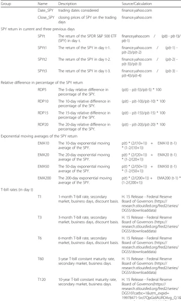
The dataset utilized in this study includes the daily direction (up or down) of the closing price of the SPDR S&P 500 ETF (ticker symbol: SPY) as the output, along with 60 financial and economic factors as input features. This daily data is collected from 2518 trading days between June 1, 2003 and May 31, 2013. The 60 potential features can be divided into 10 groups, including the SPY return for the current day and the three previous days, the rela-tive difference in percentage of the SPY return, the exponential moving averages of the SPY return, Treasury bill (T-bill) rates, certificate of deposit rates, financial and economic indicators, term and default spreads, exchange rates between the USD and four other cur-rencies, the return of seven major world indices (other than the S&P 500), the SPY trading volume, and the return of eight large capitalization companies within the S&P 500 (which is a market cap weighted index and driven by the larger capitalization companies within the index). These features, which are a mixture of those identified by various researchers (Cao & Tay,2001; Thawornwong & Enke,2004; Armano, Marchesi, & Murru,2005; Enke & Thawornwong,2005; Niaki & Hoseinzade,2013; and Zhong & Enke,2017a,2017b), are included as long as their values are released without a gap of more than five continuous trading days during the study period. The details of these 60 financial and economic fac-tors, including their descriptions, sources, and calculation formulas, are given in Table10

(4)

Data preprocessing

Data normalization

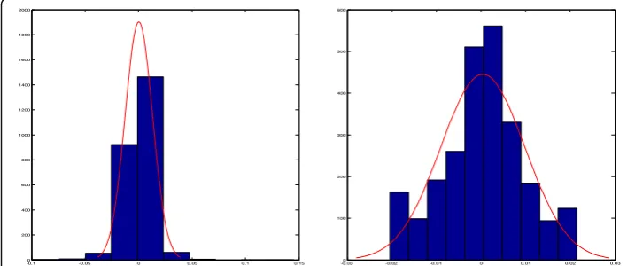
Given that the data used in this study cover 60 factors over 2518 trading days, there invariably exist missing values, mismatching samples, and outliers. Yet, the data quality is an important factor that can make a difference in the prediction accuracy, and therefore, preprocessing the raw data is necessary. Using the 2518 trading days during the 10-year period, the collected samples from other days are initially deleted. If there arenvalues for any variable or column that are continuously missing, the average of thenexisting values on both sides of the missing values are used to fill in the n missing values. A simple but classical statistical principle is employed to detect the possible outliers (Navidi,2011). The possible outliers are then adjusted using a similar method to the one used by Cao & Tay (2001). Specifically, for each of the 60 factors or columns in the data, any value beyond the interval (Q1−1.5∗IQR,Q3+ 1.5∗IQR) is regarded as a possible outlier, with the factor value replaced by the closer boundary of the interval. Here,Q1andQ3are the first and third quartiles, respectively, of all the values in that column, andIQR=Q3−Q1is the interquartile of those values. The symmetry of all adjusted and cleaned columns can be checked using histograms or statistical tests. For example, Fig-ure1 includes the histograms of factor SPYt(i.e., the SPY current daily return), before and after data preprocessing (Zhong & Enke,2017a). It can be observed that the outliers are re-moved, and the symmetry is achieved after adjustments.

In this study, the ANNs and DNNs for pattern recognition are used as the classi-fiers. At the start of the classification mining procedure, the cleaned data are sequen-tially partitioned into three parts: training data (the first 70% of the data), validation data (the last 15% of the first 85% of the data), and the testing data (the last 15% of the data).

Data transformation using PCA

As one of the earliest multivariate techniques, PCA aims to construct a low-dimensional rep-resentation of the data while maintaining the maximal variance and covariance structure of the data (Jolliffe,1986). To achieve this goal, a linear mappingWthat can maximizeWTvar( X)W, where var(X) is the variance-covariance matrix of the data X, needs to be created. Given that Wis formed by the principal eigenvectors of var(X), PCA turns out to be an

eigenproblem var(X)W=λW, where λ represents the eigenvalues of var(X). It is also

(5)

known that working on the raw dataXinstead of the standardized data with the PCA tends to emphasize variables that have higher variances more than variables that have very low var-iances, especially if the units where the variables are measured are inconsistent. In this study, not all variables are measured at the same units. Thus, here, PCA is actually applied to the standardized version of the cleaned dataX. The specific procedure is given below.

First, the linear mappingW∗is searched such that

corrð ÞX W¼λW; ð1Þ

and corr(X) is the correlation matrix of the data X. Assume that the data Xhas the format X= (X₁X₂⋯X_M); then corr(X) =ρ is aM×M matrix, where M is the dimen-sionality of the data, and theijthelement of the correlation matrix is

corrXi;Xj¼ρij¼

σij

σiσj;

where.

σij¼ covXi;Xj;σi¼

ffiffiffiffiffiffiffiffiffiffiffiffiffiffiffiffiffi varð ÞXi p

;σj¼

ffiffiffiffiffiffiffiffiffiffiffiffiffiffiffiffiffiffi var Xj q

;andi;j¼1;2;…;M: ð2Þ

Let λ¼fλ_igM_i_¼1 denote the eigenvalues of the correlation matrixcorr(X) such that λ1≥λ

2≥⋯≥λ

M and the vectors eTi ¼ ðei1ei2⋯eiMÞ denote the eigenvectors of corr(X)

corresponding to the eigenvalues λ_i,i= 1, 2,…,M. The elements of these eigenvec-tors can be proven to be the coefficients of the principal components.

Secondly, the principal components of the standardized data are presented as

Z¼ðZ1Z2⋯ZMÞ;

where.

ZT

w ¼ðZ1wZ2w⋯ZNwÞ;Zvw¼Xvw_σ−μw w ;v

¼1;2;…;N;andw¼1;2;…;M ð3Þ

can be written as.

Yi¼

X_M

j¼1eijZj;i¼1;2;…;M ð4Þ

Using the spectral decomposition theorem,

ρ¼XM

i¼1

λ

ieieTi ð5Þ

and the fact that eT_i ei ¼PMj¼1e2ij¼1 and the different eigenvectors are perpendicular

to each other such that eT_iej¼0, we can prove that

varð Þ ¼Yi XM

k¼1

XM

l¼1

eikcorrðXk;XlÞeil¼ eTi ρei¼λi ð6Þ

and

covYi;Yj¼ XM

k¼1

XM

l¼1

eikcorrðXk;XlÞejl¼eTiρej¼0: ð7Þ

(6)

In summary, the principal components can be written as the linear combinations of all the factors with the corresponding coefficients equaling the elements of the eigen-vectors. Different amounts of principal components can explain different proportions of the variance-covariance structure of the data. The eigenvalues can be used to rank the eigenvectors based on how much of the data variation is captured by each princi-pal component.

Theoretically, the information loss due to the dimensionality reduction of the data

space from M tokis insignificant if the proportion of the variation explained by the

firstkprincipal components is large enough. In practice, the chosen principle

compo-nents must be those that best explain the data while simplifying the data structure as much as possible.

Neural networks for pattern recognition

Recognized as one of the most important machine learning technologies, ANNs can be viewed as a cascading model of cell types emulating the human brain by carefully defining and designing the network architecture, including the number of network layers, the types of connections among the network layers, the numbers of neurons in each layer, the learning algorithm, the learning rate, the weights among neurons, and the various neuron activation functions. All these parameters are typically determined empirically during the learning or training phase of the neural network modeling. Thus, it is usually not easy to interpret the symbolic meaning of the trained results. However, the neural networks have high tolerance for noisy data and perform very well in recognizing the different patterns of new data during the testing stage. Also, some efficient algorithms have recently been developed to extract the classification rules from the trained neural networks. The backpropagation algorithm is well ac-cepted as the most popular neural network learning algorithm, which is often carried out using a multilayer feed-forward neural network.

Multilayer feed-forward neural networks

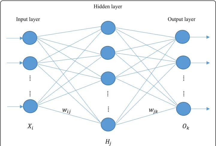
Among the various types of neural networks that have been developed, the multilayer feed-forward network is most commonly used for pattern recognition, including clas-sification, in data mining. Such a feed-forward neural network is illustrated in Fig.2.

(7)

Traditional feed-forward ANNs often utilize the backpropagation learning algorithm (Rumelhart,et al.,1986) based on an iterative process where the connection weights between the layers are adjusted repeatedly in a backwards direction, from the output layer, through the hidden layers, and then to the first hidden layer, such that the difference between the predicted class and the true class measured by the mean squared error (MSE) can be minimized during the procedure. Although other sophisticated learning algorithms have been developed over the years for specific applications, the traditional backpropagation learning is still often used to train newly developed DNNs.

DNNs for classification

More recently, deep learning, also known as deep structured learning, hierarchical learn-ing, or deep machine learnlearn-ing, has emerged as a promising branch of machine learning based on a set of algorithms that attempt to model high-level abstractions in data by using a deep graph with multiple processing layers composed of numerous linear and nonlinear transformations. This concept was introduced to the machine learning community by Dechter (1986), and later to those working with ANNs (Aizenberg et al.,2000). Researchers in this area attempt to develop better representations and models for learning these repre-sentations from large-scale unlabeled data, compared to shallow learning, where the num-ber of hidden layers is usually not greater than 10.

Since the first functional DNNs using a learning algorithm called the group method of data handling are published by Ivakhnenko (1973) and his research group, a large number of DNN architectures, such as pattern recognition networks, convolutional neural net-works, recurrent neural netnet-works, and long short-term memory, have been explored. Be-cause more hidden layers and neurons are involved in DNNs, the computational power of DNNs is expected to be higher than traditional ANNs. However, DNNs, like ANNs, suffer

(8)

from overfitting, which results from the estimation of a large number of parameters used to define the connections among hidden layers and neurons involved in DNNs, thereby re-ducing the model’s generalization ability.

Forecasting daily return direction of the SPDR S&P 500 ETF

This study focuses on predicting the daily return direction of the SPDR S&P 500 ETF (ticker symbol: SPY) for the next day. The direction forecast can be either up or down. A direction forecast (up or down) is used instead of a level forecast since this study’s objective is to not only develop a forecasting model with high classification accuracy, but also de-velop a model that can be used successfully in a practical trading environment. Previous studies (e.g., Thawornwong & Enke,2004) have shown that when developing forecasting/ trading systems, direction forecasts (up or down) perform better in a trading environment/ simulation than level forecasts (predicting the exact value of the stock or index one period forward). While level forecasts can result in models with higher reported training/testing prediction accuracy (greater than 90% in some instances), often these models are over-fitted to the data to achieve these results. Consequently, such models are more likely to suffer in a trading environment/simulation. On the other hand, since a small miss is still a miss (e.g., predicting up but being slightly down), successful direction forecasts are more likely to have a prediction accuracy closer to 60%; yet, these models still perform better at these accuracy levels when simulating real-world trading since the results from these models are more likely to be on the right side of the trade. Therefore, the following model-ing focuses on makmodel-ing an accurate and ideally profitable direction forecast.

For the model testing, three different datasets are employed, with or without the use of a PCA transformation. Trading simulations of return versus risk for the best models are discussed later.

Use of ANN and DNN classifiers

(9)

when the model suffers from overfitting, resulting in the need for the training phase to be terminated. Thus, the model can be best trained in the sense that the validation phase achieves its lowest MSE with the trained model. After the model is trained and selected, all training data, validation data, and testing data (untouched) are provided as inputs and clas-sified by the trained model separately. The percentage of correctly predicted or clasclas-sified daily directions corresponding to each category can be obtained and recorded.

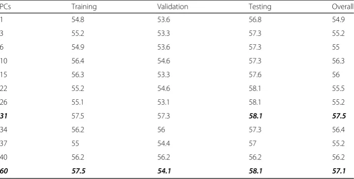
Table1shows the classification results of the traditional benchmark ANN using 12 trans-formed datasets. It shows that the benchmark ANN classifier achieves the highest accuracy in the testing phase over the PCA-represented dataset with 31 principal components; the PCA-represented dataset with 60 principal components gives the second best results.

Three datasets are considered for the DNN analysis. The first dataset includes the entire preprocessed but untransformed data, including 60 factors. The second and third datasets are transformed datasets using PCA, with 60 and 31 principal components, respectively (i.e., data with PCA equal to 60 and 31 are used since the benchmark ANN classifier achieves the highest accuracy levels in the testing phase when using the PCA-represented datasets with 31 and 60 principal components). The three sets of classification results (i.e., untransformed data, PCA = 60 data, and PCA = 31 data using both the benchmark ANN and DNN classifiers) are listed in Tables2,3and4, respectively. Please note that in Tables

2,3and4, the first row with the number of hidden layers equal to 10 represents the per-formance of the traditional benchmark feed-forward ANN.

Comparison of classification results

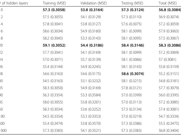
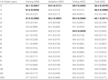
Once again, the first row in Tables 2,3and4provides the classification results using the benchmark ANN classifier (with 10 hidden layer neurons), while the remaining rows pro-vide the results from the various DNN classifiers (with the number of hidden layers greater than 10). In each of the three tables, it can be observed that as the number of hidden layers increases from 12 to 28, the accuracy of the classification in the testing phase typically in-creases, reaching the highest values of 58.6 (in Table2), 59.9 (in Table3), and 59.9 (in Table

4) when the number of hidden layers equals 28, 16, and 22, respectively. However, after the number of hidden layers becomes larger than 30 or 35, the accuracy of the classification

Table 1The ANN classification results using 12 transformed datasets

PCs Training Validation Testing Overall

1 54.8 53.6 56.8 54.9

3 55.2 53.3 57.3 55.2

6 54.9 53.6 57.3 55

10 56.4 54.6 57.3 56.3

15 56.3 53.3 57.6 56

22 55.2 54.6 58.1 55.5

26 55.1 53.1 58.1 55.2

31 57.5 57.3 58.1 57.5

34 56.2 56 57.3 56.4

37 55 54.4 57 55.2

40 56.2 56.2 56.2 56.2

(10)

for the testing data stops climbing and drops or converges to values that are close to the results using the ANN classifiers (which includes 10 hidden layers), except for one case where the transformed data with PCs = 60 and the number of hidden layers = 500 is con-sidered. Note that the overfitting issue appears to be under control, in part since all the ANN and DNN classifiers are strictly trained with the same criteria, such that for each classifier the four correction percentages of the classification, corresponding to the train-ing, validation, testtrain-ing, and entire data sets cannot be significantly different from each other; that is, the absolute value of the percentage difference must be within a defined threshold, for example, 5% (Zhong & Enke,2017a,2017b).

It is also observed that after the data are transformed via PCA, the average classification accuracy in the testing phase increases significantly. Moreover, the DNN-based classifica-tion using the transformed data with PCs = 31 achieves the highest average accuracy. To verify the phenomena in a statistical manner, a set of pairedt-tests at the significance level of 0.05 are conducted and the test results are given in Table5.

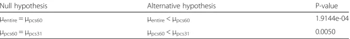
Since the P-values of the paired_t-tests are much less than 0.05, we reject the null hy-potheses and conclude that when using the DNN classifiers, the transformed dataset with PCs = 31 produces the highest average classification accuracy, while the DNN classifiers show the poorest performance over the entire preprocessed and untransformed dataset at the significance level of 0.05. Note that the values inside the parentheses in Tables2,3and

4represent the MSEs for each classification. In general, the higher the correctness percent-age, the smaller the corresponding MSEs.

Simulation

While a higher classification accuracy for a financial forecast should lead to better trading results, this is not always the case. Therefore, in this section, a trading Table 2Classification results with ANN/DNN classifiers using entire untransformed data

(11)

Table 3Classification results with ANN/DNN classifiers using transformed data with PCs = 60

# of hidden layers training (MSE) validation (MSE) testing (MSE) total (MSE) 10 58.2 (0.3062) 54.1 (0.3110) 57.8 (0.3091) 57.5 (0.3074) 12 56.9 (0.3079) 53.3 (0.3137) 58.1 (0.3066) 56.6 (0.3086) 14 57.9 (0.3041) 54.6 (0.3135) 57.8 (0.3084) 57.4 (0.3062) 16 59.4 (0.3020) 55.4 (0.3128) 59.9 (0.3056) 58.9 (0.3042) 18 56.7 (0.3071) 54.6 (0.3109) 58.9 (0.3089) 56.7 (0.3080) 20 58.8 (0.3052) 54.4 (0.3109) 59.2 (0.3074) 58.2 (0.3064) 22 57.3 (0.3065) 55.4 (0.3133) 59.4 (0.3083) 57.3 (0.3078) 24 56.9 (0.3080) 54.9 (0.3099) 58.4 (0.3082) 56.8 (0.3083) 26 55.9 (0.3101) 56.0 (0.3105) 58.4 (0.3088) 56.3 (0.3099) 28 57.8 (0.3057) 56.5 (0.3105) 59.4 (0.3079) 57.9 (0.3067) 30 56.2 (0.3076) 53.6 (0.3152) 58.1 (0.3104) 56.1 (0.3092) 35 56.6 (0.3066) 56.2 (0.3134) 58.1 (0.3081) 56.8 (0.3078) 40 59.8 (0.2999) 54.9 (0.3125) 57.6 (0.3095) 58.7 (0.3032) 45 56.3 (0.3096) 54.6 (0.3163) 57.3 (0.3113) 56.2 (0.3109) 50 55.2 (0.3103) 53.6 (0.3154) 57.3 (0.3078) 55.3 (0.3107) 100 56.9 (0.3077) 53.1 (0.3205) 57.6 (0.3221) 56.4 (0.3117) 500 55.5 (0.3345) 54.9 (0.3309) 59.9 (0.3162) 56.1 (0.3312) 1000 58.4 (0.3240) 55.7 (0.3392) 58.1 (0.3285) 57.9 (0.3269)

Table 4Classification results with ANN/DNN classifiers using transformed data with PCs = 31

(12)

simulation is conducted to see if the higher prediction accuracy from the DNN classi-fiers indicates higher profitability among the three datasets with different representa-tion. This study is based on predicting the direction of the SPDR S&P 500 ETF (ticker symbol: SPY) daily returns. Consequently, we modify the trading strategy for classifi-cation models defined by Enke & Thawornwong (2005) as follows.

If UPt+ 1= 1, fully invest in stocks or maintain, and receive the actual stock return for the day t+ 1 (i.e., SPYt+ 1); if UPt+ 1= 0, fully invest in one-month T-bills or main-tain, and receive the actual one-month T-bill return for the dayt+ 1 (i.e., T1Ht+ 1).

Here UP denotes the SPY daily return direction as predicted by the models

de-scribed earlier. In addition, the actual one-month T-bill return for the dayt+ 1 is

T1H_tþ1¼discount rate100term360days¼T1tþ1

100

28days 360days¼

T1_tþ1

100

7 90; ð8Þ

where T1t+ 1 is the one-month T-bill discount rate (or risk-free rate) percentage on

the secondary market for business day t+ 1. The original data for T1 are obtained

from the St. Louis Federal Reserve Economic Research database (https://fred.

stlouisfed.org/series/TB4WK) and are exactly the “4-week” T-bill discount rate per-centage on the secondary market; the data are listed on the website as “Monthly” in terms of the“Frequency”feature of the data but is a 28-day measure.

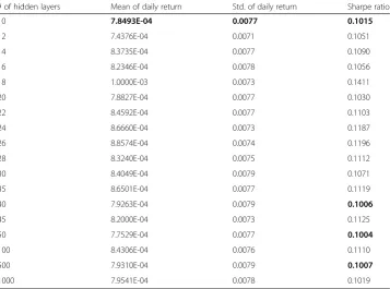
In practice, at the beginning of each trading day, the investor decides to buy the SPY portfolio or the one-month T-bill according to the forecasted direction of the SPY daily return. It is assumed for this research that the money invested in either a stock portfolio or T-bills is illiquid and detained in each asset during the entire trad-ing day. Dividends and transaction costs are also not considered. In addition, for this study, both leveraging and short selling when investing are forbidden. The trading simulation is done for all the classification models over each testing period, including 376 samples of the three data sets considered; the first day of the 377-day testing period is excluded owing to the lack of a direction prediction for that day. The result-ing mean, standard deviation (or volatility), and Sharpe ratio of the daily returns on investment generated from each forecasting model over each set of testing data are then calculated, with or without the PCA involved. The Sharpe ratio is obtained by dividing the mean daily return by the standard deviation of the daily returns. There-fore, the higher the Sharpe ratio, as a result of a higher mean daily return and/or a lower standard deviation or volatility of daily returns, the better the trading strategy. The relevant results are presented in Tables6,7and8.

As shown in Table6, the trading strategies based on the DNN classifiers for the en-tire untransformed data generate higher Sharpe ratios than the trading strategy based on the ANN classifier, except for three cases where the number of hidden layers is 40,

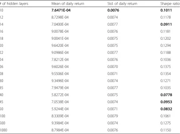
50, or 500. In Table 7, the trading strategies from the DNN classification over the

PCA-represented data with PCs = 60 result in higher Sharpe ratios than the ANN-based trading strategy, except when the number of hidden layers equals 14, 40, Table 5Comparison of classification results from DNN classifiers for three data sets

Null hypothesis Alternative hypothesis P-value

μentire=μpcs60 μentire<μpcs60 1.9144e-04

(13)

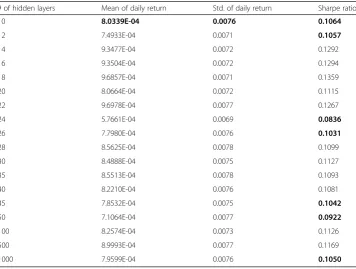
45, or 50. Table8shows that the Sharpe ratios that are generated by the trading strat-egies using the DNN classification over the PCA-represented data with PCs = 31 are mostly higher than the Sharpe ratios generated by the ANN-based trading strategy, except for those cases where the number of hidden layers is 12, 24, 26, 45, 50, or 1000. The Sharpe ratios and their corresponding hidden layer numbers that are rele-vant to these exceptions are highlighted in Tables6,7and8.

To compare the three sets of Sharpe ratios (17 values in each set) that are obtained from the trading strategies based on the DNN classifiers for the entire untransformed data and the PCA-represented data with PCs = 60 and PCs = 31, another group of paired t-tests are performed at the significance level of 0.05. TheP-values of the tests are included in Table9.

Since the P-values are all much larger than 0.05, we have strong evidence of insig-nificant differences among the mean Sharpe ratios from the three different trading strategies at the significance level of 0.05. However, with more careful observation of these P-values (and using other significance levels, e.g., 0.40), it is reasonable to con-clude that in general the trading strategies guided by the DNN classification based on the PCA-represented data perform slightly better than the ones based on the entire untransformed data, although these trading strategies perform similarly.

Conclusions and suggestions for future work

A comprehensive big data analytics procedure using hybrid machine learning algo-rithms has been developed to forecast the daily return direction of the SPDR S&P 500 ETF (ticker symbol: SPY). Ideally, researchers look to apply the simplest set of Table 6Simulation results with ANN/DNN classifiers using entire untransformed data

# of hidden layers Mean of daily return Std. of daily return Sharpe ratio

10 7.8493E-04 0.0077 0.1015

12 7.4376E-04 0.0071 0.1051

14 8.3735E-04 0.0077 0.1090

16 8.2346E-04 0.0078 0.1056

18 1.0000E-03 0.0073 0.1411

20 7.8827E-04 0.0077 0.1030

22 8.4592E-04 0.0077 0.1103

24 8.6660E-04 0.0073 0.1187

26 8.8574E-04 0.0074 0.1196

28 8.3240E-04 0.0075 0.1112

30 8.4049E-04 0.0079 0.1071

35 8.6501E-04 0.0077 0.1119

40 7.9263E-04 0.0079 0.1006

45 8.2000E-04 0.0073 0.1125

50 7.7529E-04 0.0077 0.1004

100 8.4306E-04 0.0076 0.1110

500 7.9310E-04 0.0079 0.1007

(14)

algorithms to the least amount of data, with both the most accurate forecasting re-sults and the highest risk-adjusted profits being desired. We have also considered this standard for this research.

The analytic process starts with data cleaning and preprocessing and concludes with an analysis of the forecasting and simulation results. The comparison of the classification and simulation results is done with statistical hypothesis tests, showing that on average, the ac-curacy of the DNN-based classification is significantly higher than the PCA-represented data over the entire untransformed data set. More specifically, the DNN-based classifica-tion for the PCA-represented data set with PCs = 31 achieves the highest accuracy. It is also observed that as the number of DNN hidden layers increases, a pattern regarding the classification accuracy (as compared to the ANN classifier) emerges, with the overfitting issue remaining under control. In addition, over three data sets with different representa-tions, the trading strategies using the DNN classifiers perform better than the ones using the ANN classifiers in most cases. Although in general there is no significant difference among the trading strategies from the DNN classification process over the entire untrans-formed data set and two PCA-represented data sets, the trading strategies based on the PCA-represented data perform slightly better.

In previous studies (Zhong & Enke,2017a,2017b), the PCA-ANN classifiers are shown to give a higher prediction accuracy for the daily return direction of the SPY ETF for the next day than the FRPCA-ANN classifiers, KPCA-ANN classifiers, and logistic regression classifiers, with or without PCA/FRPCA/KPCA involved. Also, the trading strategies based on the PCA-ANN classifiers perform better than the other strategies based on the other classifiers. Moreover, when using PCA, all classification model-based trading strategies per-form better than the benchmark one-month T-bill strategy; the trading strategies from the Table 7Simulation results with ANN/DNN classifiers using transformed data with PCs = 60

10 7.6471E-04 0.0076 0.1011

12 8.7298E-04 0.0074 0.1178

14 7.0400E-04 0.0077 0.0911

16 9.0078E-04 0.0076 0.1181

18 9.0041E-04 0.0075 0.1202

20 9.6420E-04 0.0075 0.1294

22 9.0986E-04 0.0077 0.1188

24 7.8212E-04 0.0076 0.1036

26 9.6026E-04 0.0070 0.1375

28 9.5506E-04 0.0071 0.1354

30 9.3496E-04 0.0074 0.1271

35 7.9479E-04 0.0077 0.1035

40 5.8272E-04 0.0075 0.0778

45 7.0538E-04 0.0074 0.0953

50 5.9244E-04 0.0071 0.0832

100 8.3309E-04 0.0079 0.1061

500 9.3984E-04 0.0074 0.1275

(15)

ANN classification mining procedure perform better than the benchmark buy-and-hold strategy. Thus, when combined with the new results as illustrated in Tables2,3,4and6,7 8it can be concluded that among the machine learning techniques considered in this study series, the PCA-DNN classifiers with the proper number of hidden layers can achieve the highest classification accuracy and result in the best trading strategy performance.

With additional hidden layers and more complicated learning algorithms, DNNs are rec-ognized as an important and advanced technology in the fields of computational intelligence and artificial intelligence. However, DNNs are still regarded as a black box with less clear theoretical confirmations of the learning algorithms that are used in common deep architectures, such as the stochastic gradient descent methodology. These DNN learning algorithms actually increase the computation time as a large number of hidden layers and neurons are included. This area of research needs to receive more attention and effort in the future.

Table 8Simulation results with ANN/DNN classifiers using transformed data with PCs = 31

10 8.0339E-04 0.0076 0.1064

12 7.4933E-04 0.0071 0.1057

14 9.3477E-04 0.0072 0.1292

16 9.3504E-04 0.0072 0.1294

18 9.6857E-04 0.0071 0.1359

20 8.0664E-04 0.0072 0.1115

22 9.6978E-04 0.0077 0.1267

24 5.7661E-04 0.0069 0.0836

26 7.7980E-04 0.0076 0.1031

28 8.5625E-04 0.0078 0.1099

30 8.4888E-04 0.0075 0.1127

35 8.5513E-04 0.0078 0.1093

40 8.2210E-04 0.0076 0.1081

45 7.8532E-04 0.0075 0.1042

50 7.1064E-04 0.0077 0.0922

100 8.2574E-04 0.0073 0.1126

500 8.9993E-04 0.0077 0.1169

1000 7.9599E-04 0.0076 0.1050

Table 9Comparison of simulation results from DNN classifiers for three data sets

Null hypothesis Alternative hypothesis P-value

μentire=μpcs60 μentire≠μpcs60 0.6251

μpcs60=μpcs31 μpcs60≠μpcs31 0.8897

μentire=μpcs31 μentire≠μpcs31 0.6635

μentire=μpcs60 μentire<μpcs60 0.3126

μpcs60=μpcs31 μpcs60<μpcs31 0.5552

(16)

Appendix

Table 10The 60 financial and economical features of the raw data

Group Name Description Source/Calculation

Date_SPY trading dates considered finance.yahoo.com Close_SPY closing prices of SPY on the trading

days

finance.yahoo.com

SPY return in current and three previous days

SPYt The return of the SPDR S&P 500 ETF (SPY) in day t.

finance.yahoo.com / (p(t) - p(t-1))/ p(t-1)

SPYt1 The return of the SPY in day t-1. finance.yahoo.com / (p(t1) -p(t-2))/p(t-2)

Relative difference in percentage of the SPY return

RDP5 The 5-day relative difference in percentage of the SPY.

(p(t) - p(t-5))/p(t-5) * 100

(p(t) - p(t-10))/p(t-10) * 100

(p(t) - p(t-15))/p(t-15) * 100

(p(t) - p(t-20))/p(t-20) * 100

Exponential moving averages of the SPY return

EMA10 The 10-day exponential moving average of the SPY.

p(t) * (2/(10+1)) + EMA10 (t-1) * (1-2/(10+1))

p(t) * (2/(20+1)) + EMA20 (t-1) * (1-2/(20+1))

p(t) * (2/(50+1)) + EMA50 (t-1) * (1-2/(50+1))

p(t) * (2/(200+1)) + EMA200 (t-1) * (1-2/(200+1))

T-bill rates (in day t)

T1 1-month T-bill rate, secondary market, business days, discount basis.

H. 15 Release - Federal Reserve Board of Governors (https:// research.stlouisfed.org/fred2/series/ DGS5/downloaddata)

T60 5-year T-bill constant maturity rate, secondary market, business days.

T120 10-year T-bill constant maturity rate, secondary market, business days.

(17)

Table 10The 60 financial and economical features of the raw data(Continued)

Certificate of deposit rates (in day t)

CD1 Average rate on 1-month neogtiable certificates of deposit (secondary market), quoted on an investment basis.

H. 15 Release - Federal Reserve Board of Governors

Financial and economical indicators (in day t)

Oil Relative change in the price of the crude oil (Cushing, OK WTI Spot Price FOB (dollars per barrel)).

Energy Inormation Administration, http://tonto.eia.doe.gov/dnav/pet/hist/ rwtcd.htm (work on cleaning the price column first using the SPY dates as control, then cal the relative change) Gold Relative change in the gold price usagold.com (use FireFox to Select

All, then copy and paste to an Excel file) (the dates used by USAGOLD are not matching with the SPY prices from yahoo.finance. For example, after 06/09/2004. We still clean/make up/delete the gold prices based on the dates of SPY prices from finance.yahoo.com. Use the same procedure in the whole data set: Take the average of the two closest data with the missing one in the middle. Then delete the mismatching one, and cal the relatvie difference as before. Another example, the data in 2011, all Friday's prices were recorded as Sunday's prices, so we estimated Friday's prices with the average of Thursday and Sunday's prices. Then deleted Sunday's prices. If there are n continuous values missing, then take the average of the n available values on each side of these n missing values, use the average for all n missing values)

CTB3M Change in the market yield on US Treasury securities at 3-month constant maturity, quoted on investment basis.

CTB6M Change in the market yield on US Treasury securities at 6-month constant maturity, quoted on investment basis.

CTB1Y Change in the market yield on US Treasury securities at 1-year constant maturity, quoted on investment basis.

CTB5Y Change in the market yield on US Treasury securities at 5-year constant maturity, quoted on investment basis.

CTB10Y Change in the market yield on US Treasury securities at 10-year

(18)

constant maturity, quoted on investment basis.

AAA Change in the Moody's yield on seasoned corporate bonds - all industries, Aaa.

BAA Change in the Moody's yield on seasoned corporate bonds - all industries, Baa.

The term and default spreads

TE1 Term spread between T120 and T1. TE1 = T120 - T1 TE2 Term spread between T120 and T3. TE2 = T120 - T3 TE3 Term spread between T120 and T6. TE3 = T120 - T6 TE5 Term spread between T3 and T1. TE5 = T3 - T1 TE6 Term spread between T6 and T1. TE6 = T6 - T1 DE1 Default spread between BAA and AAA. DE1 = BAA - AAA DE2 Default spread between BAA and

T120.

DE2 = BAA - T120

DE4 Default spread between BAA and T6. DE4 = BAA - T6 DE5 Default spread between BAA and T3. DE5 = BAA - T3 DE6 Default spread between BAA and T1. DE6 = BAA - T1 DE7 Default spread between CD6 and T6. DE7 = CD6 - T6 Exchange rate between USD and four other currencies (in day t)

USD_Y Relative change in the exchange rate between US dollar and Japanese yen.

http://www.investing.com/ currencies/usd-jpy-historical-data

USD_GBP Relative change in the exchange rate between US dollar and British pound.

http://www.investing.com/currencies/ gbp-usd-historical-data (then, take the opposites to the changes)

USD_CAD Relative change in the exchange rate between US dollar and Canadian dollar.

http://www.investing.com/ currencies/usd-cad-historical-data USD_CNY Relative change in the exchange rate

between US dollar and Chinese Yuan (Renminbi).

http://www.investing.com/ currencies/usd-cny-historical-data

The return of the other seven world major indices (in day t)

HSI Hang Seng index return in day t. finance.yahoo.com SSE

Composite

Shang Hai Stock Exchange Composite index return in day t.

finance.yahoo.com

FCHI CAC 40 index return in day t. finance.yahoo.com FTSE FTSE 100 index return in day t. finance.yahoo.com GDAXI DAX index return in day t. finance.yahoo.com DJI Dow Jones Industrial Average index

return in day t.

finance.yahoo.com(no download function for this one);

measuringworth.com/datasets/DJA/ result.php

IXIC NASDAQ Composite index return in day t.

finance.yahoo.com

SPY trading volume (in day t)

V Relative change in the trading volume of S&P 500 index (SPY)

finance.yahoo.com

The return of the eight big companies in S&P 500 (in day t)

(19)

Abbreviations

ANN:Artificial Neural Network; DNN: Deep Neural Network; PCA: Principal Component Analysis

Acknowledgements

The authors would like to acknowledge the Laboratory for Investment and Financial Engineering and the Department of Engineering Management and Systems Engineering at the Missouri University of Science and Technology for their financial support and the use of their facilities.

Funding

Post-doctoral funding was provided for Dr. Xiao Zhong by the Department of Engineering Management and Systems Engineering at the Missouri University of Science and Technology.

Availability of data and materials

Upon publication, publication data will be made available athttp://web.mst.edu/~enke/main_publications.htmland/or the Missouri University of Science and Technology Scholars Mine data repository (http://scholarsmine.mst.edu/).

Authors’contributions

XZ contributed to the neural network model development and coding, input dataset preprocessing, model testing, and trading simulation. DE contributed to the neural network model development, input data selection, and trading strategy development. Both authors read and approved the final manuscript.

Authors’information

Dr. Xiao Zhong ([email protected]) received her B.S. in Computer Software, her Ph.D. in Computer Science and Technology, her M.S. in Applied Statistics and Financial Mathematics, and a Ph.D. in Mathematics with emphasis in Statistics from Shandong University in 1994, Zhejiang University in 2001, Worcester Polytechnic Institute in 2004 and 2010, and the Missouri University of Science and Technology in 2015, respectively. She worked as a postdoctoral associate at the Department of Computer Science and Technology of Tsinghua University and Whitehead Institute of Massachusetts Institute of Technology, as well as within the Laboratory for Investment and Financial Engineering at Missouri S&T. Dr. Zhong is currently a Visiting Assistant Professor at Clark University. Her research interests include artificial intelligence, pattern recognition, data mining, and statistical applications in finance, economics, engineering, and biology.

Dr. David Enke ([email protected]) received his B.S. in Electrical Engineering and M.S. and Ph.D. in Engineering Management, all from the University of Missouri - Rolla. He is a Professor of Engineering Management and Systems Engineering at the Missouri University of Science and Technology, as well as the director of the Laboratory for Investment and Financial Engineering. His research interests are in the areas of investments, derivatives, financial engineering, financial risk management, portfolio management, algorithmic trading, hedge funds, financial forecasting, volatility forecasting, neural network modeling and computational intelligence. He has published over 100 journal articles, book chapters, refereed conference proceedings and edited books, primarily in the above research areas.

Ethics approval and consent to participate

Both authors give their approval and consent to participate.

Consent for publication

Both authors give their consent for publication.

Competing interests

The authors declare that they have no competing interests.

Publisher’s Note

Springer Nature remains neutral with regard to jurisdictional claims in published maps and institutional affiliations.

Author details 1

Graduate School of Management, Clark University, 313B Carlson Hall, 950 Main Street, Worcester, MA 01610, USA.

2_{Laboratory for Investment and Financial Engineering, Department of Engineering Management and Systems}

XOM Exxon Mobil stock return in day t. finance.yahoo.com GE General Electric stock return in day t. finance.yahoo.com JNJ Johnson and Johnson stock return in

day t.

finance.yahoo.com

WFC Wells Fargo stock return in day t. finance.yahoo.com AMZN Amazon.com Inc stock return in day t. finance.yahoo.com JPM JPMorgan Chase & Co stock return in

day t.

(20)

Engineering, Missouri University of Science and Technology, 221 Engineering Management, 600 W. 14th Street, Rolla, MO 65409-0370, USA.

Received: 26 June 2018 Accepted: 17 April 2019

References

Aizenberg I, Aizenberg NN, Vandewalle JPL (2000) Multi-Valued and Universal Binary Neurons: Theory, Learning and Applications. Springer Science & Business Media, Boston

Amornwattana S, Enke D, Dagli C (2007) A hybrid options pricing model using a neural network for estimating volatility. Int J Gen Syst 36(5):558–573

Armano G, Marchesi M, Murru A (2005) A hybrid genetic-neural architecture for stock indexes forecasting. Inf Sci 170(1):3–33 Atsalakis GS, Valavanis KP (2009) Surveying stock market forecasting techniques–part II: soft computing methods. Expert

Syst Appl 36(3):5941–5950

Bogullu VK, Enke D, Dagli C (2002) Using neural networks and technical indicators for generating stock trading signals. Intell Eng Syst Art Neural Networks, Am Soc Mechanical Eng 12:721–726

Cao L, Tay F (2001) Financial forecasting using vector machines. Neural Comput & Applic 10:184–192

Chen AS, Leung MT, Daouk H (2003) Application of neural networks to an emerging financial market: forecasting and trading the Taiwan stock index. Comput Oper Res 30(6):901–923

Chiang WC, Enke D, Wu T, Wang R (2016) An adaptive stock index trading decision support system. Expert Syst Appl 59:195–207 Chong E, Han C, Park FC (2017) Deep learning networks for stock market analysis and prediction: methodology, data

representations, and case studies. Expert Syst Appl 83:187–205

Chun SH, Kim SH (2004) Data mining for financial prediction and trading: application to single and multiple markets. Expert Syst Appl 26(2):131–139

Dechter R (1986) Learning while searching in constraint-satisfaction problems. AAAI-86 Proceedings, Palo Alto, pp 178–183 Enke D, Mehdiyev N (2013) Stock market prediction using a combination of stepwise regression analysis, differential

evolution-based fuzzy clustering, and a fuzzy inference neural network. Intell Autom Soft Comput 19(4):636–648 Enke D, Thawornwong S (2005) The use of data mining and neural networks for forecasting stock market returns. Expert Syst

Appl 29(4):927–940

Hansen JV, Nelson RD (2002) Data mining of time series using stacked generalizers. Neurocomputing 43(1–4):173–184 Huang Y, Kou G (2014) A kernel entropy manifold learning approach for financial data analysis. Decis Support Syst 64:31–42 Huang Y, Kou G, Peng Y (2017) Nonlinear manifold learning for early warning in financial markets. Eur J Oper Res 258(2):692–702 Hussain AJ, Knowles A, Lisboa PJG, El-Deredy W (2007) Financial time series prediction using polynomial pipelined neural

networks. Expert Syst Appl 35:1186–1199

Ivakhnenko AG (1973) Cybernetic predicting devices. CCM Information Corporation, Amsterdam Jolliffe T (1986) Principal component analysis. Springer-Verlag, New York

Kim KJ, Han I (2000) Genetic algorithms approach to feature discretization in artificial neural networks for the predication of stock price index. Expert Syst Appl 19(2):125–132

Kim YM, Enke D (2016) Developing a rule change trading system for the futures market using rough set analysis. Expert Syst Appl 59:165–173

Lam M (2004) Neural network techniques for financial performance prediction: integrating fundamental and technical analysis. Decis Support Syst 37:567–581

Navidi W (2011) Statistics for engineers and scientists, 3rd edn. McGraw-Hill, New York

Nayak SC, Misra BB (2018) Estimating stock closing indices using a GA-weighted condensed polynomial neural network. Financ Innov 4(21):1–22

Niaki STA, Hoseinzade S (2013) Forecasting S&P 500 index using artificial neural networks and design of experiments. J Indust Eng Int 9(1):1–9

Refenes APN, Burgess AN, Bentz Y (1997) Neural networks in financial engineering: a study in methodology. IEEE Trans Neural Netw 8(6):1222–1267

Rumelhart DE, Hinton GE, Williams RJ (1986) Learning representations by back-propagating errors. Nature 323(6088):533–536 Shen L, Loh HT (2004) Applying rough sets to market timing decisions. Decis Support Syst 37(4):583–597

Sorzano, C. O. S., Vargas, J., & Pascual-Montano, A. (2014). A survey of dimensionality reduction techniques. arXiv: 1403.2877v1 [stat.ML]

Thawornwong S, Dagli C, Enke D (2001) Using neural networks and technical analysis indicators for predicting stock trends.

Intelligent Engineering Systems through Artificial Neural Networks. Am Soc Mech Eng 11:739–744

Thawornwong S, Enke D (2004) The adaptive selection of financial and economic variables for use with artificial neural networks. Neurocomputing 56:205–232

Ture M, Kurt I (2006) Comparison of four different time series methods to forecast hepatitis a virus infection. Expert Syst Appl 31(1):41–46 van der Maaten LJ, Postma EO, van den Herik HJ (2009) Dimensionality reduction: a comparative review. J Mach Learn Res

10(1–41):66–71

Vanstone B, Finnie G (2009) An empirical methodology for developing stock market trading systems using artificial neural networks. Expert Syst Appl 36(3):6668–6680

Vellido A, Lisboa PJG, Meehan K (1999) Segmentation of the on-line shopping market using neural networks. Expert Syst Appl 17(4):303–314

Wang YF (2002) Predicting stock price using fuzzy grey prediction system. Expert Syst Appl 22(1):33–39

Zhang G (2003) Time series forecasting using a hybrid ARIMA and neural network model. Neurocomputing 50:159–175 Zhang G, Patuwo BE, Hu MY (1998) Forecasting with artificial neural networks: the state of the art. Int J Forecast 14(1):35–62 Zhong X, Enke D (2017a) Forecasting daily stock market return using dimensionality reduction. Expert Syst Appl 67:126–139 Zhong X, Enke D (2017b) A comprehensive cluster and classification mining procedure for daily stock market return