R E S E A R C H A R T I C L E
Open Access
High-resolution simulations of turbidity
currents
Edward Biegert, Bernhard Vowinckel, Raphael Ouillon and Eckart Meiburg
*Abstract
We employ direct numerical simulations of the three-dimensional Navier-Stokes equations, based on a continuum formulation for the sediment concentration, to investigate the physics of turbidity currents in complex situations, such as when they interact with seafloor topography, submarine engineering infrastructure and stratified ambients. In order to obtain a more accurate representation of the dynamics of erosion and resuspension, we have furthermore developed a grain-resolving simulation approach for representing the flow in the high-concentration region near and within the sediment bed. In these simulations, the Navier-Stokes flow around each particle and within the pore spaces of the sediment bed is resolved by means of an immersed boundary method, with the particle-particle interactions being taken into account via a detailed collision model.
Keywords: Turbidity currents, Navier-Stokes simulations, Continuum formulation, Grain-resolving simulations
Introduction
Turbidity currents are particle-laden flows in the ocean that are driven by gravity (Meiburg and Kneller 2010). Par-ticle concentrations are usually sufficiently low far away from the sediment bed so that particle-particle interac-tions play a small or negligible role throughout most of the body of the current. In this region, the Boussinesq approximation of the Navier-Stokes equations, in con-junction with a continuum formulation for the sediment concentration, is well-suited to capture the dynamics of the flow. However, near the sediment bed particle concen-trations can be very high, which can potentially result in complex non-Newtonian behavior, hindered settling, and other effects. Here, we describe the above two different simulation approaches, along with representative results, which open up a path towards multiscale flow simulations via theμ(I)rheology (Cassar et al. 2005; Boyer et al. 2011; Aussillous et al. 2013).
Methods
Continuum approach
Physical model and governing equations
In many situations of interest, compositional gravity cur-rents and turbidity curcur-rents are driven by small density
*Correspondence: [email protected]
Department of Mechanical Engineering, University of California, Santa Barbara, Engineering II, Santa Barbara, CA 93106, USA
differences not exceedingO(1%). Under such conditions, the Boussinesq approximation can be employed, which treats the density as constant in the momentum equation with the exception of the body force terms. When deal-ing with turbidity currents, we account for the dispersed particle phase by means of a Eulerian-Eulerian formula-tion, which means that we employ a continuum equation for the particle concentration field, rather than tracking particles individually in a Lagrangian fashion.
In the following, it will be important to carefully distin-guish between dimensional and dimensionless variables. Towards this end, we will employ the tilde symbol to indi-cate a dimensional variable, whereas variables without the tilde symbol are dimensionless. Under the Boussinesq approximation, the dimensional governing equations for compositional gravity currents driven by salinity and/or temperature gradients can be written as
∂uj ∂xj =
0, (1)
∂ui ∂t +
∂uiuj
∂xj = −
1
ρ1
∂p ∂xi +ν
∂2u
i ∂xj∂xj +
ρg ρ1
egi, (2)
∂ρ ∂t +
∂ρuj
∂xj = α ∂2ρ
∂xj∂xj
. (3)
Here,uidenotes the velocity vector,pthe pressure,ρthe
density,gthe gravitational acceleration,egi the unit vector
g=g ρ1 −ρ2 ρ1
. (5)
whereρ2represents the ambient density. After nondimen-sionalization, we obtain
∂uj ∂xj =
0, (6)
∂ui ∂t +
∂uiuj
∂xj = − ∂p ∂xi +
1 Re
∂2u
i ∂xj∂xj +ρ
egi, (7)
∂ρ ∂t +
∂ρuj
∂xj =
1 ReSc
∂2ρ
∂xj∂xj
. (8)
Here, the nondimensional pressurepand densityρare given by
p= p
ρ1u2b
, ρ= ρ−ρ2
ρ1 −ρ2
. (9)
The nondimensionlization of the governing equations gives rise to two dimensionless parameters in the form of the Reynolds numberReand the Schmidt numberSc
Re=ubH 2ν , Sc=
ν
α . (10)
While the Reynolds number indicates the ratio of iner-tial to viscous forces, the Schmidt number represents the ratio of kinematic fluid viscosity to molecular diffusivity of the density field.
When the driving density difference is due to gradients in particle loading, rather than salinity or temperature gradients, the above set of equations no longer provides a full description of the flow. Particles settle within the fluid, so that the scalar concentration field no longer moves with the fluid velocity. In addition, particle-particle interactions can result in such effects as hindered set-tling (Ham and Homsy 1988), increased effective viscos-ity, and non-Newtonian dynamics (Guazzelli and Morris 2011), thereby further complicating the picture. How-ever, away from the sediment bed, turbidity currents are often quite dilute, with the volume fraction of the sus-pended sediment phase being well below O(1%). Under such conditions, particle-particle interactions can usually be neglected, so that the particle settling velocity remains
scale of the flow, such as the Kolmogorov scale in turbu-lent flow. In addition, we consider only particles whose aerodynamic response timetpis significantly smaller than
the smallest time scale of the flowtf, so that the particle Stokes number St =tp/tf O(1) (Raju and Meiburg
1995). Here, the aerodynamic response time is defined as
tp= ρpd2p
18μ , (11)
with ρp indicating the particle material density and μ
denoting the dynamic viscosity of the fluid. Such particles can then be assumed to move with a velocityup,ithat is
obtained by superimposing the local fluid velocityuiand
the particle settling velocityusegi
up,i=ui+usegi , (12)
whereus follows from balancing the gravitational force
with the Stokes drag force
Fi =3πμdp(ui−up,i) (13)
as
us=
d2p(ρp−ρ)g
18μ . (14)
Note that this implies that the particle velocity field is single-valued and divergence-free, so that monodisperse particles do not, for example, accumulate near stagna-tion points or get ejected from vortex centers. Hence, we can describe the spatio-temporal evolution of the particle number concentration fieldcin a Eulerian fashion by the transport equation
∂c ∂t+
∂cuj+usegj
∂xj =α ∂2c
∂xj∂xj
. (15)
The diffusion term in Eq. (15) represents a model for the decay of concentration gradients due to the hydrodynamic diffusion of particles and/or slight variations in particle size and shape (Davis and Hassen 1988; Ham and Homsy 1988).
drag force acting on the particles. In a dimensional form, these equations read
∂uj ∂xj =
0, (16)
∂ui ∂t +
∂uiuj
∂xj = −
1
ρ
∂p ∂xi +ν
∂2u
i ∂xj∂xj +
c
ρFi, (17)
As we had done for compositional gravity currents, we use the domain half heightH/2 and buoyancy velocityub
for nondimensionalization. The reduced gravityg appear-ing in the calculation ofub can now be calculated as
g= π(ρp−ρ)c0 d3p
6ρ g, (18)
wherec0indicates a reference number concentration of particles in the suspension. After nondimensionalization, we obtain
∂uj ∂xj =
0 , (19)
∂ui ∂t +
∂uiuj
∂xj =− ∂p ∂xi+
1 Re
∂2u
i ∂xj∂xj+
cegi, (20)
∂c ∂t +
∂cuj+usegj
∂xj =
1 ReSc
∂2c
∂xj∂xj
. (21)
For polydisperse suspensions containing particles of dif-ferent sizes, the above approach can easily be extended by solving one concentration equation for each particle size and corresponding settling velocity (Nasr-Azadani and Meiburg 2014). Note that the set of governing equations for turbidity currents (19)–(21) differs from the corre-sponding set for compositional gravity currents (6)–(8) only by the additional settling velocity term in the concen-tration equation. In the following, we employ Eqs. (19)– (21) for both types of currents, with the tacit assumption that the settling velocity vanishes for compositional grav-ity currents.
Direct numerical simulations (DNS) represent the most accurate computational approach for studying gravity cur-rents. In DNS, all scales of motion, from the integral scales dictated by the boundary conditions down to the dissipative Kolmogorov scale determined by viscosity, are explicitly resolved. However, for the case of turbidity cur-rents, when the particle diameter is smaller than the Kolmogorov scale, the fluid motion around each particle is usually not resolved, due to the prohibitive computational cost. Nevertheless, the drag law accurately captures the exchange of momentum between the two phases at scales smaller than the Kolmogorov scale, so that the approach described above is still referred to as DNS.
Consistent with the above arguments, the grid spacing required for DNS is of the order of the Kolmogorov scale, while the time step needs to be of the same order as the
time scales of the smallest eddies. Due to the large dis-parity between integral and Kolmogorov scales at high Reynolds numbers, the computational cost of DNS scales asRe3, so that the DNS approach is effectively limited to laboratory scale Reynolds numbers. The first DNS simula-tions of gravity currents in a lock-exchange configuration were reported by Härtel et al. (2000) forRe = 1225. Necker et al. (2002) extended this work to turbidity cur-rents atRe = 2240. More recent simulations of lock-exchange gravity currents by Cantero et al. (2008) were able to reachRe = 15, 000, which corresponds to a lab-oratory scale current of height 0.5 m with a front velocity of 3 cm/s.
DNS simulations can provide detailed information on the structure and statistics of the flow, on the various com-ponents of its energy budget, on the mixing behavior, and many additional aspects. As a case in point, the simula-tions by Härtel et al. (2000) explored the detailed flow topology near the current front and demonstrated that the stagnation point is located a significant distance behind the nose of the current. DNS results are furthermore very useful for testing the accuracy and identifying any defi-ciencies in larger-scale LES and RANS models (Yeh et al. 2013). Thus, while they are currently limited to labora-tory scale currents, DNS simulations represent an excel-lent research tool for exploring the detailed physics of moderate Reynolds number gravity currents and for con-structing larger-scale models for higher Reynolds number applications.
Results and discussion
Continuum approach results
We illustrate the ability of the continuum approach to reproduce lab-scale experiments by presenting the results of highly resolved simulations of a turbidity current mov-ing down a slope into a stratified saline ambient. The numerical setup directly replicates the experiments con-ducted by Snow and Sutherland (2014) and is presented in Fig. 1. The density inside the ambient increases linearly fromρT at the top toρBat the bottom such that
ρ2(y)=ρB+(ρT−ρB)· y
H (22)
The channel has a constant width denoted asW. The lock region is initially at rest with densityρ1, chosen such thatρB > ρ1 > ρT. Att = 0, the lock is released and
the particle-laden flow moves down the slope forming a turbidity current interacting with the ambient fluid. Here, both the particle concentrationcand salinityscontribute to the Boussinesq term in Eq. (20) such that Eq. (21) has to be solved for each scalar field, withus = 0 in the case of
Fig. 1Problem setup and configuration.aParticle-laden fluid.bAmbient stratified fluid.cSolid region.HandLdenote the height and length of the ramp,Ldis the horizontal length of the domain,h0andLldenote the height and horizontal length of the lock, andmis the slope.ρ1is the bulk density of the lock,ρTis the initial density at the top of the ambient,ρBis the initial density at the bottom of the ambient, andρAis the initial density
in the ambient at half-lock depth
We define a nondimensional buoyancy frequency N to quantify stratification such that
N=
˜
ρ0(ρ˜B− ˜ρT) ˜
ρT(ρ˜1− ˜ρA) ˜ H ˜ h0
, (23)
whereρ˜0is a reference density.
A finite difference code is used to solve the equations, and the MPI library is used for parallelization. A third-order Runge-Kutta scheme with a three substep method is used to discretize the equations in time. The wall-normal viscous and diffusive terms are solved implicitly while the convective terms and the remaining viscous and diffusive terms are treated explicitly. To impose incompressibility, a projection method is used (Spalart et al. 1991) and a direct solver is used for the resulting Poisson equation. Slip-wall boundary conditions are used at the top and right walls andz-periodic boundary conditions are used at the lateral walls. The domain is assumed to be sufficiently long to neglect boundary effects inx, and the width of the domain is chosen so that the periodic boundary condition does not impact the flow development. Finally, an immersed boundary method is used to impose the no-slip condition on the slope (Nasr-Azadani and Meiburg 2011).
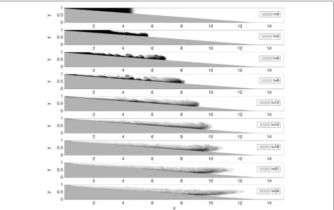
In Fig. 2, we present a time series depicting the evolu-tion of a typical turbidity current moving down a slope and intruding when its density matches that of the stratified ambient. The spanwise-averaged particle concentration is represented on a linear gray scale for various times. Upon release of the lock, the current starts moving down the slope and a trail of large Kelvin-Helmholtz rollers forms in the tail. These large instabilities then break into fully three-dimensional turbulence creating smaller dissipative vortices (t > 10). The absence of large distinct structures indicates the presence of fully developed turbulence in the tail of the current.
The direct impact of stratification is seen at later times (t ≈ 15) when the current intrudes into the ambient,
i.e. separates from the surface of the slope. The effects of stratification on intrusion depth are key in understanding the evolution of the suspended mass, deposition profiles and energy budgets of turbidity currents. Intrusion only occurs when the density of the current reaches the density of the ambient.
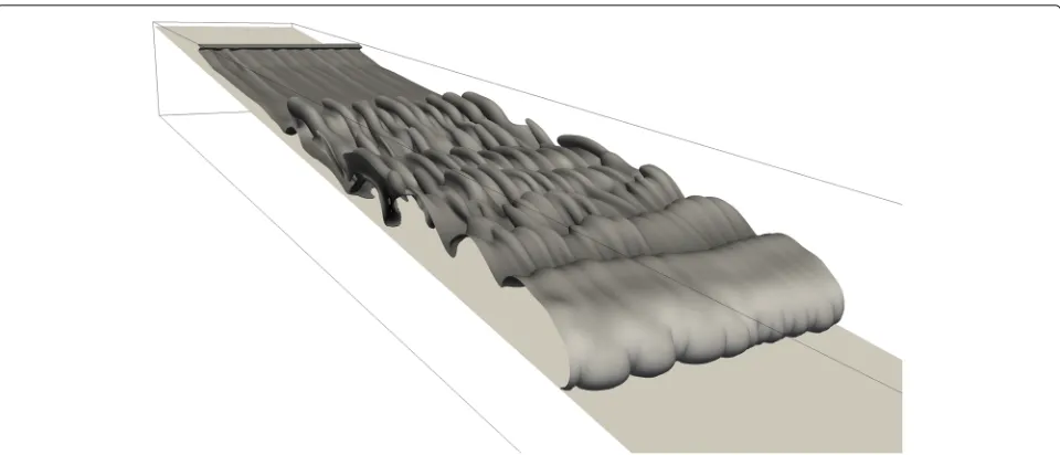
Using numerical simulations, we are able to investigate the fundamental mechanisms that control the propaga-tion of the turbidity current and monitor all the relevant dynamic variables. For instance, we can investigate the ini-tial perturbation that leads to the spanwise breakdown of the large Kelvin-Helmoltz structures that initially appear in the tail of the current. Figure 3 is a representation of the concentration isosurface c = 0.25 at t1 = 10 for a typical turbidity current at Re = 6000. The flow at that instant is not yet fully turbulent but displays strong spanwise instabilities characterized at the head by the lobe-and-cleft instability. This instability is respon-sible for the breakdown of the large Kelvin-Helmholtz rollers that only high-resolution 3D simulations are able to capture.
Fig. 2Spanwise averaged particle concentration pseudo-color plot for various times (Re = 15000,vs = 0.001,N = 2.11,m = 0.0744). This
represents the case of a turbidity current with non-zero settling velocity moving down a uniformly stratified ambient. The density of the lock is initially larger than the ambient fluid outside of the lock such that the current starts moving downslope upon release. It then encounters region of denser and denser saline ambient, until its density reaches that of the ambient and it intrudes horizontally. The flow is 2D at very early stages but quickly grows unstable under the effect of a spanwise instability at the head. This leads to the breakdown of 2D vorticies into much smaller 3D mixing structures at the head and all along the body of the current at the interface with the ambient
corresponds to a relative error of 0.8% when compared to the analytical result.
The depth at which the current intrudes into the ambi-ent also reveals a good agreemambi-ent between the two approaches and validates the ability of numerical sim-ulations to reproduce the dynamical features of turbid-ity currents moving into a stratified ambient. While it is extremely challenging to experimentally measure the velocity, particle concentration, and salinity fields of such 3D turbulent flows, direct numerical simulations give access to an entirely new set of data and opens the door to more accurate prediction tools and a deeper under-standing of the underlying physics of gravity and turbidity currents in realistic environments at the scale of the lab.
Methods
Grain-resolving approach
Physical model and governing equations
When the concentration of particles grows large, particle-particle interactions become important and the aforemen-tioned continuum approach is no longer applicable. For
Fig. 3Concentration isosurfacec = 0.25 att = 10 (Re = 6000,vs = 0.005,N = 2.09,m= 0.0744). The iso-surface reveals the global structure
of the envelope of a hyperpycnal current upon destibalization. The lobe-and-cleft instability is clearly visible at the head of the current as hills and crests form in the spanwise direction. This instability propagates in the body of the current and destabilises the large 2D vortical structures initially present. The largest wavelength corresponds to the initial dominant mode of the instability and dictates the width of the domain necessary to observe the instability at this given Reynolds number
use grain-resolved simulations to develop better models of sediment transport to be used in larger-scale simulations. We employ an immersed boundary method (IBM) developed by Uhlmann (2005) and Kempe and Fröhlich (2012) with a modified collision model adjusted for the present context, as explained below. This method solves the Navier-Stokes equations everywhere in the domain, including nearby and within the particles:
∂u
∂t + ∇ ·(uu)= − 1
ρf ∇p+νf∇
2u+fIBM (24)
where ρf is the fluid density andfIBM is the IBM force,
which acts as a source term to enforce the no-slip condi-tion at the particle surfaces. This force effectively couples the particle and fluid momentum equations. Though there are many ways to carry out this coupling, the method we employ for the particles uses regularized Dirac delta func-tions, which interpolate fluid velocities onto the particle surface and spreadfIBMonto the fluid (Roma et al. 1999).
Table 1Comparison of numerically and experimentally measured front velocity
Exp 1 Exp 2 Exp 3
Re 16,850 15,000 35,000
N 3.66 2.39 2.77
vs 0.001 0.0046 0.00046
(Ue −Us)/Ue 14% −11% 16%
Data from Snow and Sutherland (2014). The experimentally measured and numerically computed front velocities are denoted asUeandUsrespectively
Note that this implementation is different from that used to create the sloped lower wall in the turbidity current simulations of the previous section.
The equations of motion for the particles are given by the momentum equations for the translational velocity
up = (up,vp,wp)T
mp
dup
dt = pτ·ndA
=Fh
+Vp(ρp−ρf)g
=Fg
+Fl+Fc, (25)
the angular velocityωp=(ωp,x,ωp,y,ωp,z)T
Ip
dωp
dt = pr×(τ·n)dA
=Th
+Tl+Tc, (26)
and the positionxp=(xp,yp,zp)T
dxp
dt =up. (27)
Here,mpis the particle mass,pthe fluid-particle
inter-face, τ the hydrodynamic stress tensor, ρp the particle
density,Vpthe particle volume,gthe gravitational
acceler-ation,Ip = 8πρpR5p/15 the moment of inertia, andRpthe
particle radius. Furthermore, the vectornis the outward-pointing normal on the interfacep, r = x − xp is
the position vector of the surface point with respect to the center of massxpof a particle,FlandTlare the force
Fh, and torque, Th, using the approach of Kempe and Fröhlich (2012), fully resolving the hydrodynamic effects of the fluid on the particles as well as the particles on the fluid. The lubrication force,Fl, and contact force,Fc,
model close-range particle-particle interactions. With the exception of the tangential lubrication force, the methods used to evaluate these forces are described and validated in detail by Biegert et al. (2017), but here, we present them briefly.
The lubrication force
Fl= − 6πρfνfReff
Reff max(ζn,ζmin)
gn+Ft∗gt
+ Fr∗(Rpωp×n+Rqωq×n)
(28)
and torque
Tl=8πρfνfR2eff
gtTt∗+Tr∗(Rpωp×n+Rqωq×n)
×n
(29)
are added to account for short-range hydrodynamic forces that are unresolved by the fluid grid. Here, Reff = RpRq/(Rp + Rq)is an effective radius accounting
for size differences between particlespandq,gnandgtare
the relative velocities in the normal and tangential direc-tions, respectively, between the two particle surfaces at the point of contact,ζn is the surface distance between the
two particles, andζn,min = 3 × 10⁻³Rpis a limiter
pre-venting the lubrication force from reaching its singularity atζn→0. The termsFt∗,Fr∗,Tt∗, andTr∗were obtained via
asymptotic expansions by Goldman et al. (1967):
Ft∗ ∼ 8 15ln
max(ζn,ζmin)
Reff
−0.9588 (30)
Fr∗ ∼ − 2 15ln
max(ζn,ζmin)
Reff
−0.2526 (31)
Tt∗ ∼ − 1 10ln
max(ζn,ζmin)
Reff
−0.1895 (32)
Tr∗ ∼ 2 5ln
max(ζn,ζmin)
Reff
−0.3817. (33)
As indicated in (25) and (26), we also account for particle-particle contacts throughFcandTc. These
con-tact forces are composed of components normal and tan-gential to the particle surface, represented byFn andFt,
respectively, which act at the point of contact between the two particles so that the resulting force and torque on the particle are given by
Fc = Fn+Ft (34) Tc = Rpn×Ft, (35)
wherenis the outward-pointing normal vector from the contact point. A nonlinear spring-dashpot model is used for the normal contact force
Fn= −kn|ζn|3/2n−dngn, (36)
where the stiffness and damping coefficients,kn anddn,
respectively, are adaptively calibrated for every collision. A linear spring-dashpot model is used for the tangential contact force
Ft=min
−ktζt−dtgt,||μFn||t
, (37)
where ζt is the tangential displacement vector repre-senting accumulated slip between the two surfaces,μis the coefficient of friction between the surfaces, and tis the unit normal vector in the tangential direction. The Coulomb friction criterion, represented by||μFn||, allows
the two surfaces to slip past one another when large stresses are present. Similar to the normal coefficients, the tangential coefficients of stiffness and damping,ktanddt,
are also adaptively calibrated.
Results and discussion
Grain-resolving results
Pressure-driven flow over dense sediment
To address the bulk behavior of a dense granular bed sheared by a laminar Poiseuille flow, we carried out numerical simulations to reproduce the experimental results of Aussillous et al. (2013), who studied pressure-driven flows over glass spheres with a mean diame-ter Dp = 1.1 mm and a standard deviation of σ(Dp) = 0.1 mm as a sediment material. This
experi-mental work provides investigations over a range of sub-mergenceshf/Dp and Reynolds numbers in the laminar
regime, where hf is the height of the clear-water layer
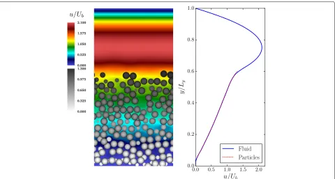
above the sediment bed illustrated in Fig. 4. We definehf
to be the height above which the average particle volume fractionφ < 0.05, which is the threshold for negligible impact of particle-particle interaction on the flow (Capart and Fraccarollo 2011).
We executed several simulations in an attempt to match the experimental results of Aussillous et al. (2013) at different flow rates and fluid heights. To this end, we sim-ulated a monodisperse granular sediment bed sheared by a pressure-driven Poiseuille flow with periodic conditions in both the streamwise (x) and spanwise (z) directions, respectively. A no-slip condition was applied at the top and bottom wall as well as at the particle surface. A detailed comparison validating the simulation results has been presented in great detail in Biegert et al. (2017). Here, we extend this work to show data from the same physi-cal setup, but with an increased flow rate, such that the gross of the particles are set into motion and interact in a complex network. The physical and numerical parameters associated with this simulation are listed in Table 2.
Fig. 4Pressure-driven flow over a dense sediment bed. The left figure shows an instantaneous slice through the domain, the color scale illustrating streamwise fluid velocity, and the gray scale illustrating particle velocity. The right figure shows the time-and-space-averaged streamwise velocity of the fluid and particles
the bulk fluid velocity Ub = L1y Ly
0 udy. In the clear-water layer, a parabolic profile obeying the analytical solu-tion of the classical Poiseuille flow can be observed. The lower end of this parabolic region, however, is not a no-slip wall, but a moving granular bed, which causes the symmetry axis of the flow profile to shift from hf/2 to
a lower position. Inside the granular bed, a linear shear flow profile develops and since all particles are moving, this profile continues all the way to the bottom wall of the domain. This interesting behavior and the wealth of data obtained from the grain-resolving simulations opens
Table 2Simulation parameters of the pressure-driven flow scenario, whereuτ =√τw/ρfis the friction velocity at the
fluid/particle interface,Ubis the bulk (average) velocity of the
fluid,τwis the shear stress at the fluid/particle interface,νfthe
kinematic viscosity,Lx,Ly, andLzare the spatial extents of the
computational domain in the Cartesian space, andhis the grid cell size
Re = UbLy/νf 9.9
D+ = uτDp/νf 0.39
Sh = τw/[(ρp−ρf)gD] 0.97
ρp/ρf 2.1
Lx × Ly × Lz 11.26Dp ×22.52Dp × 11.26Dp
hf/Dp 8.7
Dp/h 22.7
up a wide range of analytical tools in terms of statistical description as well as physical modeling, which will be our focus in the future.
Shearing of dense suspensions
To further investigate the rheologic properties of dense suspensions, we simulated a shear flow of two parallel walls with a spacing ofHmoving in opposite directions. A no-slip condition is applied for the moving walls at the top and bottom of the domain and at the particle surface. The walls move with a relative velocityUw = Ut −Ub,
whereUtis the velocity of the top wall andUbis the
veloc-ity of the bottom wall. Periodic conditions are applied in streamwise (x) and spanwise (z) directions. The fluid in between the two walls is a dense mixture of spheri-cal particles, where “dense” indicates a volume fraction φv = NpVp/Vf > 0.4. Here,Vp = 4πR3p/3 is the
volume of a single particle,Npis the number of particles
in the computational domain Vf, and Rp is the
parti-cle radius. The dimension of the computational domain can be treated as part of the physical problem. We have considered two computational domains: scenario A with
Table 3Physical and numerical simulation parameters for simulations of shear flows with dense suspensions
edry μk μs ν ζmin ρp/ρf H/Dp Dp/h Re
Table 4Simulation scenarios
Scenario Lx × Ly × Lz Re φv ts˙I ta˙I
Re10p42 2H × 1H × 1H 10 0.42 85 35 Re10p54 2H × 1H × 1H 10 0.54 150 30 Re40p54 1H × 2H × 1H 40 0.54 20 20
dimensionsLx × Ly × Lz = 2H × 1H × 1H and
scenario B withLx × Ly × Lz = 1H × 2H × 1H.
Thus, the relative submergence becomesH/Dp = 10
andH/Dp = 20, respectively, whereDp is the
parti-cle diameter. For both scenarios A and B, the shear rate ˙
I = Uw/H was kept constant so that the particle
Reynolds number Rep = ˙ID2p/νf = 0.1 also stays
constant but the channel Reynolds number for scenario B is increased by a factor of 4 with respect to scenario A. This yields channel Reynolds numbers ofRe = 10 (scenario A) andRe = 40 (scenario B). The particles have a density ofρp/ρf = 1.011, which is close to
neu-trally buoyant conditions. We assume material parameters corresponding to glass or silicate materials as thoroughly validated in Biegert et al. (2017). In particular, we choose edry = 0.97,μk = 0.15,μs = 0.8, andν = 0.22,
where edry is the wall-normal restitution coefficient for
dry collisions,μkandμsare the kinetic and static friction
coefficients for oblique collisions, andνis Poisson’s ratio. Every particle is discretized by 25.6 grid cells per diam-eter. The particle parameters are summarized in Table 3. Three simulations were conducted with varying volume fractions of the mixture and different relative gap sizes H/Dpto explore the effects of these two parameters. All
simulations were initialized and run for a start-up timets
until a true steady steady state had been established. Sub-sequently, data was collected for the averaging timetato
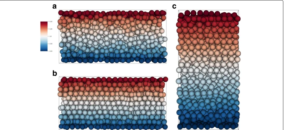
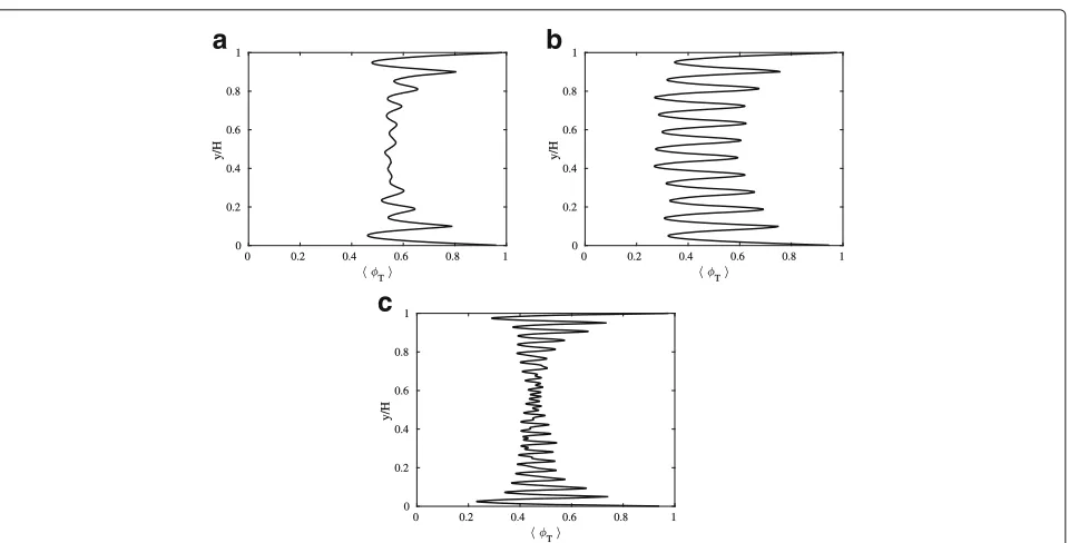
reach converged statistics for the profiles presented in the following. The different scenarios are displayed in Table 4. An instantaneous snapshot of the particle distribution colored by the particle velocity is given in Fig. 5. As desired, particles are dragged along the moving walls whenever they collide with them. These particles mov-ing with the wall transfer kinetic energy through collisions towards the channel center. In addition, the moving walls establish a background profile for the fluid velocity, which should be close to the linear shear profile commonly observed in Couette-type flows. The two mechanisms from collision and hydrodynamic interactions establish a shear flow profile within the suspension. Looking at the wall-normal profiles of the porosity, we can see a distinct pattern of oscillations (Fig. 6). This crystal-like layering of the particles reflects the fact that all particles are the same size. While a strongly layered structure is visible for all three simulations close to the wall, less pronounced layers form in the channel center for the two scenariosRe10p42 andRe40p54. For these two scenarios, particles have more space to rearrange due to the lower volume fraction and the larger relative gap size, respectively. Horizontal-and-time-averaged profiles of the streamwise component of the fluid and particle velocity show that particles move with almost the same velocity as the fluid flow (Fig. 7). Slight distortions can be seen, especially for caseRe10p54, illustrating local effects of the particle clustering on the global velocity profile.
Fig. 5Shearing of dense suspensions. Color bar indicates streamwise velocity of particles. Shown are instantaneous snapshots foraRe = 10 and
Fig. 6Porosity profiles averaged in the streamwise and spanwise directions and time for the three simulation scenarios:aRe= 10 andφv = 0.42,
bRe = 10 andφv = 0.54, andcRe = 40 andφv = 0.54
The present study of a Couette-type flow supple-ments our simulations of pressure-driven flow described in the previous section to fully understand the rheo-logic behavior of dense suspensions of particles with different inertia in flows with different momentum supply.
Internal waves propagating over fully resolved sediment beds We also studied the hydrodynamic forces acting on a fully resolved sediment bed induced by a gravity current. Here, the key issue is to explore how a jump in the hydrostatic pressure traveling along the surface of the sediment bed propagates within the bed. To this end,
a
c
b
Fig. 7Average streamwise particle velocity profiles for the three simulation scenarios:aRe = 10 andφv = 0.42,bRe= 10 andφv = 0.54, and
we solved the advection-diffusion Eq. (8) and supple-mented (24) with the term stemming from the Boussinesq approximation. The Peclet number was chosen to be Pe = ReSc = 104. The initial configuration is sim-ilar to a lock-exchange, but the particles are submerged in a layer of high concentration as well. The geometry is Lx/H × Ly/H × Lz/H = 6 × 1 × 1, whereH is
the channel height from the no-slip wall on the bottom to the free-slip wall on the top, which is equivalent toLy.
The Reynolds number for the present scenario was cho-sen to beRe = ubh/νf = 164, whereub =
ghis the buoyancy velocity,his the lock height,g= ρpρ−ρf
f gis
the specific gravity, andgis the gravitational acceleration. Free-slip walls were applied to the left, back, and front wall (Fig. 8a). The right boundary was set to be a con-vective outflow condition. The relative submergence of a particle isH/Dp = 10. Every particle is discretized by Dp/h = 16.
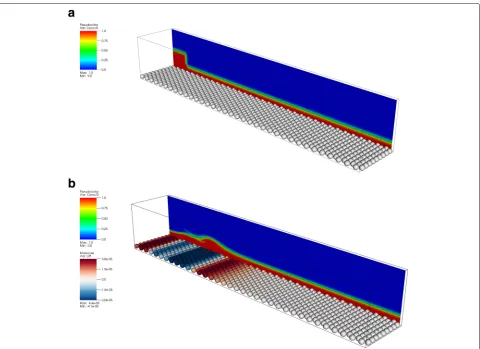
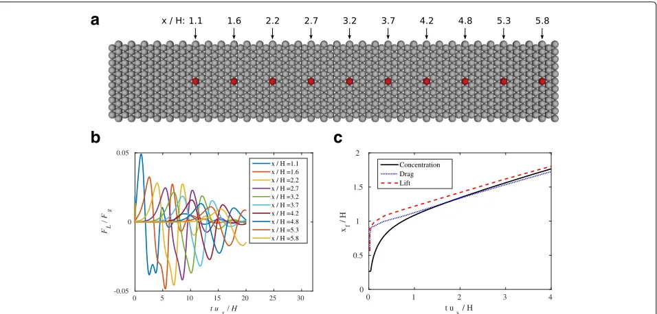
Immediately after being released, the block of heavy fluid starts to propagate along the rough wall, form-ing an internal wave at the interface between light and heavy fluid, which are indicated in Fig. 8 as blue and red fluid, respectively. Particles in Fig. 8b are colored by the lift forces acting in a vertical direction. We can see that particle in front of the wave start to experi-ence a lift force even though the wave front has not yet reached it. The grain-resolving simulation approach now allows us to track the drag and lift on individual par-ticles as a function of time to elucidate this effect in more detail. This has been done for the particles col-ored in red in Fig. 9a. The lift force normalized by the buoyant weight of the particles Fg = ρfVpg
is shown in Fig. 9b. Every curve represents a particle shown in Fig. 9a, and it becomes obvious that the lift experienced by the particles along the transect appears to be similar with decaying intensity along the flow direction.
Fig. 8Instantaneous snapshots for the internal wave study. Fixed particles are arranged in a hexagonal packing immersed in the heavy (red) fluid.
t u
s/ H
0 1 2 3 4
xf
/ H
0 0.5 1
Fig. 9Lift/drag of the internal propagating wave acting on the centerline particles.ashows a top view of the particle bed, where lift forces are measured at the red-colored centerline particles.bshows the lift force normalized by the gravitational force,FL/FG, versus time for the centerline
particles, each particle represented by a separate curve.cshows the position of the internal wave front versus time, where the position is determined either from the concentration profile, the drag force acting on the particle bed, or the lift force acting on the particle bed
We can track the front of the current using the location in the horizontal profile where the interface between light and heavy fluid starts to increase in height. Alternatively, we can track the front using the location where particles start to experience an enhanced lift force. A comparison of these two methods is shown in Fig. 9c for the first few time units simulated. It can be seen that, indeed, during the ini-tial stage of the simulation, where we can see a steep front of the internal wave, the force signal propagates quicker through the sediment bed than the actual propagation speed of the current would suggest. This effect, however, levels off over time as the wave continues to travel over the rough bed, constantly losing energy due to viscous dissipation.
Conclusions
The modeling of dilute, non-eroding turbidity currents has reached a mature level, as evidenced by the fact that high-resolution simulations have been able to repro-duce many of the observations made in laboratory exper-iments (e.g., Nasr-Azadani et al. 2013). We are now able to account for some topographical complexity via the immersed boundary method. Some of the remain-ing challenges concern the extension to the very large Reynolds number values of field-scale flows and the frequent interaction with ambient phenomena in the ocean such as internal waves and tides, as well as the accurate modeling of erosion and resuspension in such high Reynolds number flows. However, a similar level of
models for use at larger scales. This multiscale approach would thus further enrich our understanding of turbidity currents.
Acknowledgements
Computational resources for this work were provided by the Extreme Science and Engineering Discovery Environment (XSEDE), supported by the National Science Foundation, USA, Grant No. TG-CTS150053.
Funding
This research is supported in part by the Department of Energy Office of Science Graduate Fellowship Program (DOE SCGF), made possible in part by the American Recovery and Reinvestment Act of 2009, administered by ORISE-ORAU under the contract no. DE-AC05-06OR23100. BV gratefully acknowledges the Feodor-Lynen scholarship provided by the Alexander von Humboldt Foundation, Germany.
Authors’ contributions
EB and BV developed the grain-resolving simulation approach. RO carried out the continuum formulation simulations. EM proposed the topic and conceived the study. All authors read and approved the final manuscript.
Competing interests
The authors declare that they have no competing interests.
Publisher’s Note
Springer Nature remains neutral with regard to jurisdictional claims in published maps and institutional affiliations.
Received: 24 June 2017 Accepted: 9 October 2017
References
Aussillous P, Chauchat J, Pailha M, Médale M, Guazzelli É (2013) Investigation of the mobile granular layer in bedload transport by laminar shearing flows. J Fluid Mech 736:594–615
Biegert E, Vowinckel B, Meiburg E (2017) A collision model for grain-resolving simulations of flows over dense, mobile, polydisperse granular sediment beds. J Comput Phys 340:105–127
Boyer F, Guazzelli É, Pouliquen O (2011) Unifying suspension and granular rheology. Phys Rev Lett 107(18):1–5
Cantero MI, Balachandar S, García MH, Bock D (2008) Turbulent structures in planar gravity currents and their influence on the flow dynamics. J Geophys Res Oceans 113(C8):1–22
Capart H, Fraccarollo L (2011) Transport layer structure in intense bed-load. Geophys Res Lett 38(20):2–7
Cassar C, Nicolas M, Pouliquen O (2005) Submarine granular flows down inclined planes. Phys Fluids 17(10):103301
Davis RH, Hassen MA (1988) Spreading of the interface at the top of a slightly polydisperse sedimenting suspension. J Fluid Mech 196:107–134 Goldman AJ, Cox RG, Brenner H (1967) Slow viscous motion of a sphere
parallel to a plane wall-I Motion through a quiescent fluid. Chem Eng Sci 22(4):637–651
Guazzelli É, Morris JF (2011) A physical introduction to suspension dynamics. Cambridge Texts in Applied Mathematics. Cambridge University Press, Cambridge
Ham JM, Homsy GM (1988) Hindered settling and hydrodynamic dispersion in quiescent sedimenting suspensions. Int J Multiphase Flow 14(5):533–546 Härtel C, Meiburg E, Necker F (2000) Analysis and direct numerical simulation of the flow at a gravity-current head. Part 1. Flow topology and front speed for slip and no-slip boundaries. J Fluid Mech 418:189–212
Kempe T, Fröhlich J (2012) An improved immersed boundary method with direct forcing for the simulation of particle laden flows. J Comput Phys 231(9):3663–3684
Kidanemariam AG, Uhlmann M (2017) Formation of sediment patterns in channel flow: minimal unstable systems and their temporal evolution. J Fluid Mech 818:716–743
Meiburg E, Kneller B (2010) Turbidity currents and their deposits. Annu Rev Fluid Mech 42:135–156
Meiburg E, Radhakrishnan S, Nasr-Azadani M (2015) Modeling gravity and turbidity currents: computational approaches and challenges. Appl Mech Rev 67(4):040802
Nasr-Azadani MM, Meiburg E (2011) TURBINS: an immersed boundary, Navier-Stokes code for the simulation of gravity and turbidity currents interacting with complex topographies. Comput Fluids 45(1, SI):14–28 Nasr-Azadani MM, Hall B, Meiburg E (2013) Polydisperse turbidity currents
propagating over complex topography: comparison of experimental and depth-resolved simulation results. Comput Geosci 53:141–153 Nasr-Azadani MM, Meiburg E (2014) Turbidity currents intracting with
three-dimensional seafloor topography. J Fluid Mech 745:409–443 Necker F, Härtel C, Kleiser L, Meiburg E (2002) High-resolution simulations of
particle-driven gravity currents. Int J Multiphase Flow 28(2):279–300 Necker F, Härtel C, Kleiser L, Meiburg E (2005) Mixing and dissipation in
particle-driven gravity currents. J Fluid Mech 545:339
Raju N, Meiburg E (1995) The accumulation and dispersion of heavy-particles in forced 2-dimensional mixing layers .2. The effect of gravity. Phys Fluids 7(6):1241–1264
Roma AM, Peskin CS, Berger MJ (1999) An adaptive version of the immersed boundary method. J Comput Phys 153(2):509–534
Snow K, Sutherland BR (2014) Particle-laden flow down a slope in uniform stratification. J Fluid Mech 755:251–273
Spalart PR, Moser RD, Rogers MM (1991) Spectral methods for the Navier-Stokes equations with one infinite and two periodic directions. J Comput Phys 96(2):297–324
Uhlmann M (2005) An immersed boundary method with direct forcing for the simulation of particulate flows. J Comput Phys 209(2):448–476
Vowinckel B, Nikora V, Kempe T, Fröhlich J (2017) Spatially-averaged momentum fluxes and stresses in flows over mobile granular beds: a DNS-based study. J Hydraulic Res 55(2):208–223