Annihilation and sources in continuum dislocation dynamics

O R I G I N A L A R T I C L E

Open Access

Annihilation and sources in continuum

dislocation dynamics

Mehran Monavari

and Michael Zaiser

*Correspondence:

[email protected] 1_{Institute of Materials Simulation} (WW8), Friedrich-Alexander University Erlangen-Nürnberg (FAU), Dr.-Mack-Str. 77, 90762 Fürth, Germany

Full list of author information is available at the end of the article

Abstract

Continuum dislocation dynamics (CDD) aims at representing the evolution of systems of curved and connected dislocation lines in terms of density-like field variables. Here we discuss how the processes of dislocation multiplication and annihilation can be described within such a framework. We show that both processes are associated with changes in the volume density of dislocation loops: dislocation annihilation needs to be envisaged in terms of the merging of dislocation loops, while conversely dislocation multiplication is associated with the generation of new loops. Both findings point towards the importance of including the volume density of loops (or ’curvature density’) as an additional field variable into continuum models of dislocation density evolution. We explicitly show how this density is affected by loop mergers and loop generation. The equations which result for the lowest order CDD theory allow us, after spatial averaging and under the assumption of unidirectional deformation, to recover the classical theory of Kocks and Mecking for the early stages of work hardening.

Keywords: Continuum dislocation dynamics, Annihilation, Dislocation sources, CDD

Introduction

Since the discovery of dislocations as carriers of plastic deformation, developing a contin-uum theory for motion and interaction of dislocations has been a challenging task. Such a theory should address two interrelated problems: how to represent in a continuum set-ting the motion of dislocations, hence the kinematics of curved and connected lines, and how to capture dislocation interactions.

The classical continuum theory of dislocation (CCT) systems dates back to Kröner (1958) and Nye (1953). This theory describes the dislocation system in terms of a rank-2 tensor fieldαdefined as the curl of the plastic distortion,α= ∇ ×βpl. The rate of the plastic distortion due to the evolution of the dislocation density tensor reads∂tβpl=v×α where the dislocation velocity vector v is defined on the dislocation lines. The time evolution ofαbecomes (Mura1963)

∂tα= ∇×[v×α] . (1)

This fundamental setting provided by the classical continuum theory of dislocation sys-tems has, over the past two decades, inspired many models (e.g. (Sedláˇcek et al. 2003; Xiang2009; Zhu and Xiang2015)). Irrespective of the specific formulation, a main charac-teristic of the CCT is that, in each elementary volume, the dislocation tensor can measure

only the minimum amount of dislocations which are necessary for geometrical compat-ibility of plastic distortion (‘geometrically necessary’ dislocations (GND)). If additional dislocations of zero net Burgers vector are present, CCT is bound to be incomplete as a plasticity theory because the ‘redundant’ dislocations contribute to the averaged plas-tic strain rate and this contribution must be accounted for. Conversely we can state that CCT is working perfectly whenever ‘redundant’ dislocations are physically absent. This condition is of course fulfilled for particular geometrical configurations, but in general cases it can be only met if the linear dimension of the elementary volume of a simulation falls below the distance over which dislocations spontaneously react and annihilate, such that ’redundant’ dislocations cannot physically exist on the scale of the simulation. This simple observation demonstrates the close connection between the problem of averaging and the problem of annihilation - a connection which we will further investigate in detail in “Annihilation” section of the present paper.

From the above argument we see that one method to deal with the averaging problem is to remain faithful to the CCT framework and simply use a very high spatial resolution. We mention, in particular, the recent formulation by El-Azab which incorporates statis-tical phenomena such as cross-slip (Xia and El-Azab2015) and time averaging (Xia et al. 2016) and has shown promising results in modelling dislocation pattern formation. This formulation is based upon a decomposition of the tensorαinto contributions of dislo-cations from the different slip systemsς in the formα = _ςρς ⊗bς wherebς is the Burgers vector of dislocations on slip systemς and the dislocation density vectorρς of these dislocations points in their local line direction. Accordingly, the evolution of the dislocation density tensor is written as∂tα =

ς∂tρς ⊗bςwith∂tρς = ∇×[vς ×ρς] where the dislocation velocitiesvς are again slip system specific. We consider a decom-position of the dislocation density tensor into slip system specific tensors as indispensable for connecting continuum crystal plasticity to dislocation physics: it is otherwise impos-sible to relate the dislocation velocityvin a meaningful manner to the physical processes controlling dislocation glide and climb, as the glide and climb directions evidently depend on the respective slip system. We therefore use a description of the dislocation system by slip system specific dislocation density vectors as the starting point of our subsequent discussion.

CCT formulated in terms of slip system specific dislocation density vectors with single-dislocation resolution is a complete and kinematically exact plasticity theory but, as the physical annihilation distance of dislocations is of the order of a few nanometers, its numerical implementation may need more rather than less degrees of freedom com-pared to a discrete dislocation dynamics model. There are nevertheless good reasons to adopt such a formulation: Density based formulations allow us to use spatio-temporally smoothed velocity fields which reduce the intermittency of dislocation motion in dis-crete simulations. Even more than long-range interactions and complex kinematics, the extreme intermittency of dislocation motion and the resulting numerical stiffness of the simulations is a main factor that makes discrete dislocation dynamics simulations computationally very expensive. Furthermore, in CCT, the elementary volume of the simulation acts as a reaction volume and thus annihilation does not need any special treatment.

then needed which can account for the presence of ’redundant’ dislocations. Some con-tinuum theories try to resolve the averaging problem by describing the microstructure by multiple dislocation density fields which each represent a specific dislocation orientation

ϕ on a slip systemς. Accordingly, all dislocations of such a partial population move in the same direction with the same local velocityvςϕ such that∂tρςϕ

≈ ∇ ×vςϕ× ρϕς. Along this line Groma, Zaiser and co-workers (Groma1997; Zaiser et al.2001; Groma et al. 2003) developed statistical approaches for evolution of 2D systems of straight, positive and negative edge dislocations. Inspired by such 2D models, Arsenlis et al. (2004); Reuber et al. (2014); Leung et al. (2015) developed 3D models by considering additional orienta-tions. However, extending the 2D approach to 3D systems where connected and curved dislocation lines can move perpendicular to their line direction while remaining topolog-ically connected is not straightforward, and most models use, for coupling the motion of dislocations of different orientations, simplified kinematic rules that cannot in general guarantee dislocation connectivity (see Monavari et al. (2016) for a detailed discussion).

The third line takes a mathematically rigorous approach towards averaged, density-based representation of generic 3D systems of curved dislocation lines density-based on the idea of envisaging dislocations in a higher dimensional phase space where densities carry additional information about their line orientation and curvature in terms of continuous orientation variablesϕ (Hochrainer2007; Hochrainer et al. 2007). In this phase space, the microstructure is described by dislocation orientation distribution functions (DODF)

ρ(r,ϕ). Tracking the evolution of a higher dimensional ρ(r,ϕ) can be a numerically challenging task. Continuum dislocation dynamics (CDD) estimates the evolution of the DODF in terms of its alignment tensor expansion series (Hochrainer2015). The compo-nents of the dislocation density alignment tensors can be envisaged as density-like fields which contain more and more detailed information about the orientation distribution of dislocations. CDD has been used to simulate various phenomena including dislocation patterning (Sandfeld and Zaiser2015; Wu et al.2017b) and co-evolution of phase and dislocation microstructure (Wu et al.2017a). The formulation in terms of alignment ten-sors has proven particularly versatile since one can formulate the elastic energy functional of the dislocation system in terms of dislocation density alignment tensors (Zaiser2015) and then use this functional to derive the dislocation velocity in a thermodynamically consistent manner (Hochrainer2016).

Continuum dislocation dynamics Conventions and notations

We describe the kinematics of the deforming body by a displacement vector fieldu. Con-sidering linearised kinematics of small deformations we use an additive decomposition of the corresponding deformation gradient into elastic and plastic parts:∇u = βel+βpl. Dislocations of Burgers vectorsbςare assumed to move only by glide (unless stated oth-erwise) and are therefore confined to their slip planes with slip plane normal vectorsnς. This motion generates a plastic shearγςin the direction of the unit slip vectorbς/bwhere bis the modulus ofbς. We use the following sign convention: A dislocation loop which expands under positive resolved shear stress is called a positive loop, the corresponding dislocation density vectorρς points in counter-clockwise direction with respect to the slip plane normalnς. Summing the plastic shear tensors of all slip systems gives the plastic distortion:βpl=_ςγςnς⊗bς/b.

On the slip system level, without loss of generality, we use a Cartesian coordinate system with unit vectorseς₁= bς/b,e3=nςande2=nς×sssς. A slip system specific Levi-Civita tensorεςwith coordinatesε_ijςis constructed by contracting the fully antisymmetric Levi-Civita operator with the slip plane normal,ε_ijς = εikjnς_k. The operationt.ες =: t⊥then rotates a vectorton the slip plane clockwise by 90◦aroundnς. In the following we drop, for brevity, the superscriptςas long as definitions and calculations pertaining to a single slip system are concerned.

The quantity which is fundamental to density based crystal plasticity models is the slip system specific dislocation density vectorρ. The modulus of this vector defines a scalar densityρ= |ρ|and the unit vectorl=ρ/ρgives the local dislocation direction. Themth order power tensor oflis defined by the recursion relationl⊗1 = l,l⊗m+1 = l⊗m⊗l. In the slip system coordinate system,lcan be expressed in terms of the orientation angle

ϕbetween the line tangent and the slip direction asl(ϕ)= cos(ϕ)e₁+sin(ϕ)e₂. When considering volume elements containing dislocations of many orientations, or ensem-bles of dislocation systems where the same material point may in different realizations be occupied by dislocations of different orientations, we express the local statistics of dislo-cation orientations in terms of the probability density functionpr(ϕ)of the orientation

angleϕwithin a volume element located at r. We denotepr(ϕ)as the local dislocation

orientation distribution function (DODF). The DODF is completely determined by the set of momentsϕnr but also by the expectation values of the power tensor serieslnr.

The latter quantities turn out to be particularly useful for setting up a kinematic theory. Specifically, the so-called dislocation density alignment tensors

ρ(n)_(r):=ρl⊗n

r =ρ

pr(ϕ)l(ϕ)⊗ndϕ. (2)

turn out to be suitable field variables for constructing a statistically averaged theory of dis-location kinematics. Components of the k-th order alignment tensorρ(k)(r)are denoted

ρa1...ak.ρ

(n)_{(r)= ρ}(n)_{(r)/ρdenotes normalization of an alignment tensor by dividing it}

Kinematic equations of continuum dislocation dynamics (CDD) theory

Hochrainer (2015) derives the hierarchy of evolution equations for dislocation density alignment tensors by first generalizing the CCT dislocation density tensor to a higher dimensional space which is the direct product of the 3D Euclidean space and the space of line directions (second-order dislocation density tensor, SODT). Kinematic evolution equations for the SODT are obtained in the framework of the calculus of differential forms and then used to derive equations for alignment tensors by spatial projection. For a general and comprehensive treatment we refer the reader to Hochrainer (2015). Here we motivate the same equations in terms of probabilistic averaging over single-valued dislocation density fields, considering the case of deformation by dislocation glide.

We start from the slip system specific Mura equation in the form

∂tρ= ∇×[v×ρ] . (3)

where for simplicity of notation we drop the slip system specific superscript ς and

we assume that the spatial resolution is sufficiently high such that the dislocation line orientationlis uniquely defined in each spatial point. If deformation occurs by crystallo-graphic slip, then the dislocation velocity vector must in this case have the local direction ev= l×n= ρ×n/ρ. This implies that the Mura equation iskinematically non-linear: writing the right-hand side out we get

∂tρ= ∇×[l×n×ρv]= ∇ × ρ×

n×ρ

|ρ| v

. (4)

where the velocity magnitudevdepends on the local stress state and possibly on disloca-tion inertia. This equadisloca-tion is non-linear even if the dislocadisloca-tion velocityvdoes not depend onρ, and this inherent kinematic non-linearity makes the equation difficult to average. To obtain an equation which is linear in a dislocation density variable and therefore can be averaged in a straightforward manner (i.e., by simply replacing the dislocation density variable by its average) is, however, possible: We note thatρ=lρand∇×l×n×l= −ε.∇, hence

∂tρ= −ε· ∇(ρv). (5)

In addition we find because ofρ⊗b= ∇ ×βplthat the plastic strain rate and the shear strain rate on the considered slip system fulfil the Orowan equation

∂tβpl=[n⊗b]ρv=[n⊗sss]∂tγ , ∂tγ =ρbv. (6)

We now need to derive an equation for the scalar densityρ. This is straightforward: we use thatρ2=ρ.ρ, hence∂tρ=(ρ/ρ)·∂tρ. After a few algebraic manipulations we obtain

∂tρ= ∇ ·(ε·ρv)+qv (7)

where we introduced the notation

q:= −ρ(∇ ·ε·l). (8)

The quantityqdefines a new independent variable. Its evolution equation is obtained from those ofρandl =ρ/ρ. After some algebra we get

∂tq= ∇ ·

vQ−ρ(2)· ∇v. (9)

where we have taken care to write the right-hand side in a form that contains density- and curvature-density like variables in a linear manner. As a consequence, on the right hand side appears a second order tensorρ(2) =ρl⊗l = ρ⊗ρ/ρ. By using the fact thatρis divergence-free,∇.ρ = ∇.(ρl)=0, we can show that the vectorQ=qε·lderives from this tensor according to Q= ∇.ρ(2).

We thus find that the equation for the curvature densityq contains a rank-2 tensor which can be envisaged as the normalized power tensor of the dislocation density vec-tor. On the next higher level, we realize that the equation forρ(2) contains higher-order curvature tensors, leading to an infinite hierarchy of equations given in full by

∂tρ= ∇ ·(vε·ρ)+v, (10)

∂tρ(n)=

−ε· ∇vρ(n−1)+(n−1)vQ(n)−(n−1)ε·ρ(n+1)· ∇v

sym, (11)

∂tq= ∇ ·

vQ(1)−ρ(2)· ∇v

, (12)

where Q(n)are auxiliary symmetric curvature tensors defined as

Q(n)=qε·l⊗ε·l⊗l⊗n−2. (13)

So far, we have simply re-written the single, kinematically non-linear Mura equation in terms of an equivalent infinite hierarchy of kinematically linear equations for an infi-nite set of dislocation density-like and curvature-density like variables. The idea behind this approach becomes evident as soon as we proceed to perform averages over volumes containing dislocations of many orientations, or over ensembles where in different real-izations the same spatial point may be occupied by dislocations of different orientations. The fact that our equations are linear in the density-like variables allows us to average them over the DODFp(ϕ)whileretaining the functional formof the equations. The aver-aging simply replaces the normalized power tensors of the dislocation density vector by their DODF-weighted averages, i.e., by the respective dislocation density alignment tensors:

ρ(n)_(r)→

pr(ϕ)ρ(n)(r)dϕ (14)

and similarly

Q(n)(r)→

pr(ϕ)Q(n)(r)dϕ. (15)

The problem remains that we now need to close the infinite hierarchy of evolution equations of the alignment tensors. A theory that uses alignment tensors of orderkcan be completely specified by the evolution equation ofqtogether with the equations for the

contained in alignment tensors up to orderk, and then use the estimated DODF to eval-uate, from Eq. (2), the missing alignment tensorρ(k+1). This allows to close the evolution equations at any desired level.

For example, closing the theory at zeroth order is tantamount to assuming a uni-form DODF for which the corresponding closure relation readsρ(1) ≈ 0. The evolution equations of CDD(0)then are simply

∂tρ=vq (16)

∂tq=0 (17)

These equations represent the expansion of a system consisting of a constant number of loops. In “CDD(0)” section we demonstrate that, after generalization to incorporate dislocation generation and annihilation, already CDD(0) provides a the-oretical foundation for describing early stages of work hardening. CDD(0) is, how-ever, a local plasticity theory and therefore can not describe phenomena that are explicitly related to spatial transport of dislocations. To correctly capture the spatial distribution of dislocations and the related fluxes in an inhomogeneous microstruc-ture one needs to consider the evolution equations of ρ and/or of ρ(2)_{. Closing the} evolution equations at the level of ρ, or of ρ(2) yields the the first order CDD(1)

and second order CDD(2) theories respectively. The DODF of these theories have a

more complex structure that allows for directional anisotropy which we discuss in Appendix4and5together with the derivation of the corresponding annihilation terms for directionally anisotropic dislocation arrangements.

Annihilation

Dynamic dislocation annihilation

If dislocation segments of opposite orientation which belong to different dislocation loops closely approach each other, they may annihilate. This process leads to a merger of the two loops. The mechanism that determines the reaction distance is different for dislocations of near-screw and near-edge orientations:

1 Two near-screw dislocations of opposite sign, gliding on two parallel planes,

annihilate by cross slip of one of them.

2 Two near-edge dislocations annihilate by spontaneous formation and

disintegration of a very narrow unstable dislocation dipole when the attractive elastic force between two dislocations exceeds the force required for dislocation climb. As opposed to screw annihilation this process generates interstitial or vacancy type point defects.

This difference results in different annihilation distances for screw and edge segments.

The dependency of the maximum annihilation distance ya between line segments on

averaging volume, which thus is directly acting as the annihilation volume for all disloca-tions. Hence, it is difficult to account for differences in the annihilation behaviour of edge and screw dislocations.

Dislocation annihilation in continuum dislocation dynamics Straight parallel dislocations

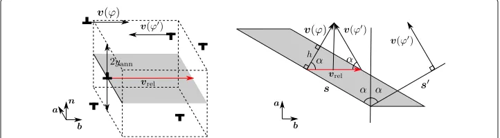
Coarse-grained continuum theories that allow for the coexistence of dislocations of dif-ferent orientations within the same volume element require a difdif-ferent approach to annihilation. Traditionally this approach has used analogies with kinetic theory where two ‘particles’ react if they meet within a reaction distanceya. Models such as the one pro-posed by Arsenlis et al. (2004) formulate a similar approach for dislocations by focusing on encounters of straight lines which annihilate once they meet within a reaction cross-section (annihilation distance) leading to bi-molecular annihilation terms (Fig.1(left)). However, dislocations are not particles, and in our opinion the problem is better formu-lated in terms of the addition of dislocation density vectors within an ’reaction volume’ that evolves as dislocations sweep along their glide planes. For didactic reasons we first consider the well-understood case of annihilation of straight parallel dislocations in these terms (Fig.1(left)). We consider positive dislocations of density vectorρ+ = eaρ+and negative dislocations of density vector ρ− = −eaρ−. During each time stepdt, each positive dislocation may undergo reactions with negative dislocations contained within a differential annihilation volumeVa = 4yavsdtwheresis the dislocation length, which for straight dislocations equals the system extension in the dislocation line direction. The factor 4 stems from the fact that the annihilation cross section is 2Ya, and the relative velocity 2v. The total annihilation volume in a reference volumeVassociated with pos-itive dislocations is obtained by multiplying this volume with the dislocation numberN+. The positive dislocation density inVisρ+=N+w/Vwherewis the average line seg-ment length. Hence, the differential annihilation volume fraction (differential annihilation volume divided by reference volume) for positive dislocations is

f_a+=Va N+

V =2yavρ

+ ₍₁₈₎

Annihilation is now simply tantamount to replacing, within the differential annihila-tion volume, the instantaneous values ofρ+andρ−by their vector sum. This summation reduces the densities of both positive and negative dislocations by the same amount. The

Fig. 1Left: Differential annihilation volume of opposite edge dislocations is determined by multiplying their

relative velocityvrel=2vw.r.t. each other with the line segment lengthwand the annihilation window 2ycb

and time step_δt:Va=4vyannwdt. Right: Similarly, differential recombination volume of segments with

orientation_ϕand_ϕ=π+ϕ−2_{αl l}is determined by multiplying their relative velocityvrel=2vcosαl l

w.r.t. the each other with the projected line segmentwcos_{αl l}which is perpendicular to relative velocity and the annihilation window 2ycband time stepδt:Va=4vyanncos2αl l

average density changes in the reference volumeV are obtained by multiplying the densities with the respective annihilation volume fractions of the opposite ’species’ and summing over positive and negative dislocations, hence

dρ+ dt =

dρ− dt = −(f

+_ρ−_+f−_ρ+_{)= −4y}

avρ+ρ−. (19)

This result is symmetrical with respect to positive and negative dislocations.

Recombination of non-parallel dislocations

Our argument based on the differential annihilation volume can be straightforwardly generalized to families of non-parallel dislocations. We first consider the case where the annihilation distance does not depend on segment orientation. We consider two fam-ilies of dislocation segments of equal length s, with directions l and l and densities

ρl andρl. The individual segments are characterized by segment vectorssss = lsand

sss=ls(for generic curved segments we simply make the transition to differential vectors dsss = ldsand dsss = lds). The segments are moving at velocityvperpendicular to their line direction (Fig.1(right)).

The argument then runs in strict analogy to the previous consideration, however, since the product of the reaction is not zero we speak of a recombination rather than an annihilation reaction. Furthermore, the differential reaction (recombination) volume is governed not by the absolute velocity of the dislocations but by the velocity at which either of the families sweeps over the other. This relative velocity is given byvrel = 2vcosαl l

where 2αl l = π−ψ andψ is the angle between the velocity vectors of both families

(Fig.1(right)). The recombination area that each segment sweeps by its relative motion to the other segment is thus given byAa=2vcosαl lsdt. The differential recombination

volume is then in analogy to Eq.18given by

f_rl=4yavcos2(αl l)ρl. (20)

Within this volume fraction we identify for each segment of directionla segment of orientationlof equal lengthsandreplacethe two segments by their vector sum (in the previously considered case of opposite segment directions, this sum is zero). Hence, we reduce, within the differential recombination volume, both densities by equal amounts and add new segments of orientation land density ρ_ls where l and s fulfil the relations:

sss=sss+sss,s= |sss|,l=sss

s (21)

We can now write out the rates of dislocation density change due to recombination as

dρl

dt = dρl

dt = −4yavρlρlcos 2_(α

l l),

dρ_l

dt =4yavρlρlcos 2_(α

l l)s(l,l). (22)

For dislocations of opposite line directions,αl l =0 ands = 0, hence, we recover the

previous expression for annihilation of parallel straight dislocations. For dislocations of the same line direction,αl l =π/2,s=2s, andl =l=l, hence, there is no change in

Recombination of loops triggered by cross slip

We now generalize our considerations to general non-straight dislocations, i.e., to ensem-bles of loops. We first observe that the relations for straight non-parallel dislocations hold locally also for curved dislocations, provided that the dislocation lines do not have sharp corners. For curved dislocations we characterize the dislocation ensemble in terms of its DODF of orientation angles, i.e., we write

l =l(ϕ)=(cosϕ, sinϕ) , ρl=ρp(ϕ),

l=l(ϕ)=(cosϕ, sinϕ) , ρ_l =ρp(ϕ), l=l(ϕ)=(cosϕ, sinϕ) , ρl=ρp(ϕ),

αl l =α(ϕ,ϕ). (23)

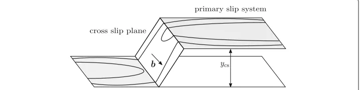
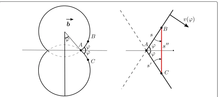
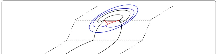
We now first consider the recombination of loops initiated by cross slip of screw disloca-tion segments. This process is of particular importance because the annihiladisloca-tion distance ycs for near-screw dislocations is almost two orders of magnitude larger than for other orientations (Pauš et al.2013). The recombination process is initiated if two near-screw segments which are oriented within a small angleϕa∈[−ϕ,ϕ] from the screw orien-tationsϕ = 0 andϕ = πpass within the distanceycs (Fig.2). Mutual interactions then cause one of the near-screw segments to cross slip and move on the cross-slip plane until it annihilates with the other segment. However, it would be erroneous to think that cross slip only affects the balance of near-screw oriented segments: Cross slip annihilation of screw segments connects two loops by a pair of segments which continue to move in the cross-slip plane. We can visualize the geometry of this process by considering the pro-jection of the resulting configuration on the primary slip plane. Figure3(left) depicts the top view of a situation some time after near-screw segments of two loops moving on par-allel slip planes have merged by cross slip. As the loops merge, the intersection pointA– which corresponds to a collinear jog in the cross slip plane that connects segments of directionl(ϕ)andl(ϕ)in the primary slip planes – moves in the Burgers vector direc-tion. Hence, the initial cross slip triggers an ongoing recombination of segments of both loops as the loops continue to expand in the primary slip system (Devincre et al.2007).

We note that the connecting segments produce slip in the cross-slip plane. The amount of this slip can be estimated by considering a situation well after the recombination event, when the resulting loop has approximately spherical shape with radiusR. The slipped area in the primary slip plane is thenπR2, and the area in the cross slip plane is, on average, Rycs/2. Hence, the ratio of the slip amount in the primary and the cross slip plane is of the order of 2πR/ycs ≈ 2πρ/(ycsq). We will show later in “CDD(0)” section that, for typical

Fig. 2Dislocation loops in a cross slip configuration. After cross slip annihilation two semi-loops are

Fig. 3Top view of a cross slip induced recombination process. Left: cross slip initiates the annihilation of near-screw segments of two merging dislocation loops. The dashed lines shows the annihilated parts of the loops. After the initiation of the cross slip, loops continue to merge by interaction between segments AB(sss(ϕ)) and AC (sss(ϕ)). Right: Recombination of segmentssss(ϕ)andsss(ϕ)generates a new segmentsss(ϕ) with edge orientation which changes the total dislocation density and mean orientation

hardening processes, the amount of slip in the cross slip plane caused by recombination processes can be safely neglected.

Comparing with Fig.1we see that, in case of cross slip induced recombination, the two recombining segments fulfil the orientation relationshipϕ = π −ϕand that the angle

αl land the length of the recombined segment are given by

αl l =ϕ, (24)

ϕ= π

2sign(π−ϕ), (25)

s= |l+l| =2|sinϕ|. (26)

We now make an important conceptual step by observing that, if two segments pertain-ing to different loops in the configuration shown in Fig.3are found at distance less than ycs, then a screw annihilation event must have taken place in the past. Hence, we can infer from the current configuration that in this case the loops are recombining. The rates for the process follow from (22) as

dρ(ϕ)

dt =

dρ(ϕ)

dt = −4ycsvρ

2_{p(ϕ)p(ϕ)cos}2_(ϕ),

dρ(ϕ)

dt =8ycsvρ

2_{p(ϕ)p(ϕ)cos}2_{(ϕ)|sinϕ|. (27)}

Multiplying (27) with the appropriate power tensors of the line orientation vectors and integrating over the orientation window where cross slip is possible gives the change of alignment tensors due to cross slip induced recombination processes:

∂tρcs(k)= −4ycsvρ2 (ϕ− |ϕ+ϕ−π|)cos2(ϕ)

l(k)(ϕ)− |sin(ϕ)|l(k)(π/2)

dϕdϕ

−4ycsvρ2 (ϕ− |ϕ+ϕ−3π|)cos2(ϕ)

l(k)(ϕ)−|sin(ϕ)|l(k)(3π/2)

dϕdϕ.

(28)

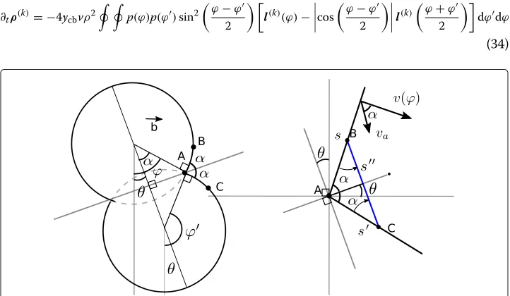
Isotropic recombination of general dislocations by climb

Next we consider recombination by climb which we suppose to be possible for dislo-cations of any orientation that are within a direction-independent cross-section 2ycbof others. Hence, the process is - unlike cross slip - isotropic in the sense that an initially isotropic orientation distribution will remain so, and recombination can occur between segments of any orientation provided they find themselves within a distance of less than ycb. To analyse this process, we focus on the plane of symmetry that bisects the angle between both segments. This plane is at an angleθ from the screw dislocation orienta-tion, see Fig.4. Now, if we rotate the picture by−θ, it is clear that the geometry of the process is exactly the same as in case of cross slip induced recombination, and that only the appropriate substitutions need to be made. The following geometrical relations hold:

θ(ϕ,ϕ)= ϕ

_+ϕ−π

2 , (29)

α(ϕ,ϕ)= ϕ−ϕ

_+π

2 , (30)

ϕ= ϕ+ϕ

2 , (31)

s=2cos

_ϕ−ϕ

2

. (32)

According to (22) the rate of recombination between segments of directionsϕandϕ then leads to the following density changes:

dρ(ϕ)

dt =

dρ(ϕ)

dt = −4yavρ

2_{p(ϕ)p(ϕ)sin}2

ϕ−ϕ

2

,

dρ(ϕ)

dt =8yavρ

2_{p(ϕ)p(ϕ)sin}2

_ϕ−ϕ

2 cos

_ϕ−ϕ

2

. (33)

Multiplying (33) with the appropriate power tensors of the line orientation vectors and integrating over all orientations gives the change of alignment tensors due to climb recombination processes:

∂tρ(k)= −4ycbvρ2 p(ϕ)p(ϕ)sin2 _ϕ−ϕ

2

l(k)(ϕ)−cos _ϕ−ϕ

2

l(k) _ϕ+ϕ

2

dϕdϕ

(34)

Fig. 4Left: Two dislocation loops are merging by climb annihilation initiated at segments with angles_θand

In particular, the rates of change of the lowest-order tensors are

∂tρ= −4ycbvρ2 p(ϕ)p(ϕ)sin2

ϕ−ϕ

2

1−cos

ϕ−ϕ

2

dϕdϕ (35)

∂tρ=0. (36)

The latter identity is immediately evident if one remembers thatρis the vector sum of all dislocation density vectors in a volume, hence, it cannot change if any two of these are added up and replaced with their sum vector.

Dynamic dislocation sources

During early stages of plastic deformation of a well-annealed crystal (ρ≈106[ m−2]), the dislocation density can increase by several orders of magnitude. This increase of disloca-tion density contributes to many different phenomena such as work hardening. Therefore, no dislocation theory is complete without adequate consideration of the multiplication problem. In CDD, multiplication in the sense of line length increase by loop expansion occurs automatically because the kinematics of curved lines requires so, however, the gen-eration of new loops is not accounted for, which leads to an incorrect hardening kinetics. In this section, we discuss several dynamic mechanisms that increase the loop density by generating new dislocation loops.

First we introduce the well-known Frank-Read source and how we formulate it in a continuous sense in the CDD framework. Frank-Read sources are fundamental parts of the cross-slip and glissile junction multiplication mechanisms which play an impor-tant role in work hardening. Therefore we use the Frank-Read source analogy to discuss the kinematic aspects of these mechanisms and the necessary steps for incorporating them into the CDD theory. We first note that the Mura equation, if applied to a FR source configuration with sufficiently high spatial resolution to a FR source, captures the source operation naturally without any further assumptions, as shown by the group of Acharya (Varadhan et al.2006). Like the problem of annihilation, the problem of sources arises in averaged theories where the spatial structure of a source can not be resolved.

To overcome this problem, Hochrainer (2007) proposed a formulation for a

continu-ous FR source distribution in the context of the higher-dimensional CDD. Sandfeld and Hochrainer (2011) described the operation of a single FR source in the context of

lowest-order CDD theory as a discrete sequence of loop nucleation events. Acharya (2001)

generalizes CCT to add a source term into the Mura equation. This term might rep-resent the nucleation of dislocation loops of finite areaex nihil which can happen at stresses close to the theoretical shear strength, or through diffusion processes which occur on relatively long time scales and lead to prismatic loops (Messerschmidt and Bartsch2003; Li2015). Neither process is relevant for the normal hardening behavior of metals.

Frank-read sources

bows out and generates a new dislocation loop and a pinned segment identical to the initial segment. Therefore, a Frank-Read source can successively generate closed disloca-tion loops Fig.5. A Frank-Read source can only emit dislocations when the shear stress is higher than a critical stress needed to overcome the maximum line tension force (Hirth and Lothe1982):

σcr≈ Gb

rFR, (37)

where the radius of the metastable loop is half the source length,rFR = L₂. The acti-vation rate of Frank-Read sources has been subject of several studies. Steif and Clifton (1979) found that in typical FCC metals, the multiplication process is controlled by the activation rate at the source, where the net driving force is minimum due to high line tension. The nucleation time can be expressed in a universal plot of dimensionless stress

σ∗ _{= σL/Gbvs dimensionless timet}∗ _{= t}

nucσb/BL, wheretnucis the nucleation time andBis the dislocation viscous drag coefficient. For a typicalσ∗ ≈ 4, the reduced time

becomes t∗ ≈ 10 (Hirth and Lothe 1982). However, this exercise may be somewhat

pointless because the stress at the source cannot be controlled from outside, rather, it is strongly influenced by local dislocation-dislocation correlations, such as the back stress from previously emitted loops. Such correlations have actually a self-regulating effect: If the velocity of dislocation motion near the source for some reason exceeds the velocity far away from the source, then the source will emit dislocations rapidly which pile up close to it and exert a back stress that shuts down the source. Conversely, if the velocity at the source is reduced, then previously emitted dislocations are convected away and the back stress decreases, such that source operation accelerates. The bottom line is, the source will synchronize its activation rate with the motions of dislocations at a distance. In our kinematic framework which averages over volumes containing many dislocations, it is thus reasonable to express the activation time in terms of the average dislocation velocity v=σb/Bas:

τ =ηrFR/v. (38)

(38) implies that the activation time is equal to the time that an average dislocation takes

to travel η times the Frank-Read source radius before a new loop can be emitted. In

Fig. 5Activation of a Frank-Read source: A dislocation segment (black) pinned at both ends bows out under

discrete dislocation dynamics (DDD) simulations, a common practice for creating the ini-tial dislocation structure is to consider a fixed number of grown-in Frank-Read sources distributed over the different slip systems (Motz et al.2009). Assuming that the length of these sources is 2rFRand the density of the source dislocations isρFR, then their volume density isnFR =ρFR/(2rFR). The activation rate is given by the inverse of the nucleation time:

νFR=v/(ηrFR). (39)

The operation of Frank-Read sources of volume density nFR increases the curvature density by 2πtimes the loop emission rate per unit volume, hence

˙

qfr=2πnFRνFR=πvρFR

ηr2_FR. (40)

We note that no corresponding terms enter the slip rates, or the evolution of the alignment tensors, which are fully described by terms characterizing motion of already generated dislocations.

Source activity has important consequences for work hardening. The newly created loops have high curvature of the order of the inverse loop radius, hence they are more effi-cient in creating line length than old loops that have been expanding for a long time. This effect of increasing the average curvature of the dislocation microstructure is of major importance for the work hardening kinetics.

Double-cross-slip sources

Koehler (1952) suggested the double-cross-slip mechanism as a similar mechanism to a Frank-Read source that can also repeatedly emit dislocation loops. In double-cross-slip, a screw segment that is gliding on the plane with maximum resolved shear stress (MRSS) and is blocked by an obstacle cross-slips to a slip plane with lower MRSS. After passing the obstacle it cross slips back to the original slip system and produces two super jogs connecting the dislocation lines. These two super-jogs may act as pinning points for the dislocation and in practice produce Frank-Read like sources (Fig.6). The double-cross-slip source is the result of the interaction of dislocations on different slip planes and therefore a dynamic process.

Several DDD studies such as Hussein et al. (2015) have tried to link the number of double-cross-slip sources in the bulk and on the boundary of grains to the total dislocation

density. They observed that the number of double-cross-slip sources increases with dislo-cation density and specimen size. However, these studies fall short of identifying an exact relation between the activation rate of cross-slip-sources and system parameters.

In the following we introduce a model for incorporating this process into CDD. The density of screw dislocationsρson a slip system is:

ρs=

_ϕ

−ϕρ(ϕ)+ _π+ϕ

π−ϕ ρ(ϕ), (41)

which in general is a function of dislocation moments functions. For the case of isotropic DODF this can be simplified toρs =4ϕ(ρ(ϕ= 0)+ρ(ϕ = π))= 4₂ϕ_π ρ. We assume that a fractionfdcsof this density is in the form of double-cross-slipped and pinned seg-ments. Hence, the source density is ndcs = ρs/rdcs, where the pinning length of the cross slipped segments is of the order of the dislocation spacing,rdcs = 1/

ρtot _with

ρtot ₌

ςρ. Otherwise we assume for the cross-slip source exactly the same relations as for the grown-in sources of densityρFRand radiusrFR. Thus, the generation rate of curvature density becomes:

˙

qdcs ≈πfdcs

η vρsρtot. (42)

The non-dimensional numbersfdcsandηcan be determined by fitting CDD data to an ensemble average of DDD simulations, or to work hardening data. While in bulk systems these parameters only depend on the crystal structure and possibly on the distribution of dislocations over the slip systems, for small systems,fdcsandηare expected to be func-tions ofρtot_l

s, the system size (e.g. grain size)lsin terms of dislocations spacing, because the source process may be modified e.g. by image interactions at the surface.

Glissile junctions

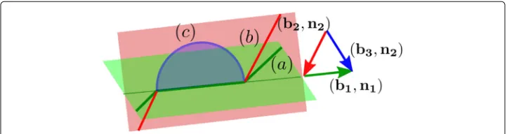
When two dislocations gliding on different slip systems (ς,ς) intersect, it can be ener-getically favourable for them to react and form a third segment called junction. Depending on the Burgers vectors and slip planes of the interacting segments this junction can be glissile (mobile) or sessile (immobile). Figure7depicts the formation of a glissile junc-tion . The segment (a) on the slip system (b₁,n₁) interacts with the segment (b) on the slip system (b₂,n₂) and together they produce the junction (c) on the slip system (b₃ = b₁+b₂,n₂) which lies on the same glide plane as the segment (b). This mech-anism produces a segment on the slip system (b3,n2) with endpoints that can move and adjust the critical stress to the applied shear stress. Recently Stricker and Weygand

Fig. 7Glissile junction reproduced from Stricker and Weygand (2015): Two dislocations on slip systems

(2015) studied the role of glissile junctions in plastic deformation. They found by consid-ering different dislocation densities, sizes and crystal orientations of samples, that glissile junctions are one of the major contributors to the total dislocation density and plastic deformation. The action of glissile junctions can be envisaged in a similar manner as the action of cross slip sources, however, we need to take into account that only a very limited number of reactions can produce a glissile junction. Suppose that two dislocations of slip systemsςandςproduce a glissile junction that can act as a source on systemς. The density of segments onςthat form junctions withςisfgjρςρς/ρtotand the length of the junctions is of the order of the dislocation spacing,rgj =1/ρtot_{. Hence we get}

˙

qς_gj≈ ς

ς

πf_gjςςvςρ ς

ρς

η . (43)

We finally note that the action of dynamic sources and recombination processes is kinematically irreversible. Consequently, by reversing the direction of the velocity, recombination mechanisms do not act as sources and vice versa.

CDD(0)

CDD(0): a model for early stages of work hardening

We now use the previous considerations to establish a model for the early stages of work hardening. In doing so we make the simplifying assumption that the ’composition’ of the dislocation arrangement, i.e. the distribution of dislocations over the different slip sys-tems, does not change in the course of work hardening. This is essentially correct for deformation in high-symmetry orientations but not for deformation in single slip con-ditions. We thus focus on one representative slip system only and assume that all other densities scale in proportion.

Since the DODF of CDD(0)is uniformρ(ϕ)= ₂ρ_π, the climb and cross slip recombi-nation rates can be combined into one set of equations:

˙

ρann= −4dannvρ2q˙ann= q

ρρ˙ann (44)

where dann is an effective annihilation distance. Although in DDD simulations, artifi-cial Frank-Read sources are often used to populate a dislocation system in early stages, we consider samples with sufficient initial dislocation density where network sources (glissile junctions) are expected to dominate dislocation multiplication. Therefore, we only consider glissile junctions in conjunction with loop generation by double-cross-slip which leads to terms of the same structure. Their contribution can be combined into one equation:

˙ qsrc=

csrc

η vρ2. (45)

Closing the kinematic Eqs. (10) and (12) at zeroth order together with the contri-bution of annihilation and sources gives the semi-phenomenological CDD(0) evolution equations:

∂tρ=qv+ ˙ρann

∂tq= ˙qann+ ˙qsrc

For quasi-static loading the sum of internal stresses should balance the applied resolved shear stress. For homogeneous dislocation microstructure the dominant internal stresses are a friction like flow stressτf ≈αbG√ρand a self interaction stress associated to line tension of curved dislocations approximated asτlt ≈ TGbq_ρ whereGdenotes the shear modulus andαandTare non dimensional parameters (Zaiser et al.2007). Therefore the applied stress becomes:

τext=τf+τlt=αbG√ρ+TGb q

ρ (47)

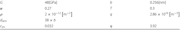
Using these relations we can build a semi-phenomenological model for work hardening. We fit the parameters of the model to the stage III hardening rate (θ = ∂τ/∂γ) of high-purity single crystal Copper during torsion obtained by Göttler (1973). Interestingly, the model captures also the stages I and II. The initial values and material properties are given in Table1.

The initial microstructure consists of a small density of low curvature dislocation loops which have low flow stress and line tension. This facilitates the free flow of disloca-tions which is the characteristic of the first stage of work hardening (marked with (I) in Fig.8-top-right). The initial growth of dislocation density is associated with expansion of dislocation loops. In this stage the curvature of microstructure w.r.t. dislocation spac-ing rapidly increases which indicates that dislocations become more and more entangled. This can be parametrized by the variable=q/(ρ)1.5as depicted by Fig.8-bottom-right. As density increases, the dynamic sources become more prominent. New dislocation loops are generated and the curvature of the system increases. In the second stage,

the hardening rate∂τ/∂γ reaches its maximum around τ = G/120. The growth rate

of dislocation density decreases which indicates the start of dynamic recovery through recombination of dislocations. In the third stage, the hardening rate decreases mono-tonically as dislocation density saturates. The late stages of hardening (IV, V) exhibit themselves as a plateau at the end of the hardening rate plot and are commonly associated with dislocation cell formation. Therefore CDD(0)cannot capture these stages. To capture these stages, one might need to use higher order non local models such as CDD(1)and CDD(2)which are cable of accounting for dislocation transport and capture cell formation (Sandfeld and Zaiser2015).

In our treatment we have neglected the slip contribution of segments that move on the cross slip plane during cross-slip induced recombination processes. We are now in a position to estimate this contribution, which we showed to be of the order offcs ≈ qycs/(2πρ)relative to the amount of slip on the primary slip plane. An upper estimate of the cross slip heightycsleading to a recombination process is provided by the dislocation

Table 1Material properties, initial values of dislocation densities of Copper

G 48[GPa] b 0.256[nm]

α 0.27 T 0.3

ρ 2×10−12_m−2 _{q 2.86×10}16_m−3

dann 38×b

Fig. 8First 3 stages of work hardening in cooper rolling. Experimental measures marked by [×] obtained from Göttler (1973). Top-left: resolved shear stress(RSS) against plastic slip. Top-right: hardening-rate vs RSS; Hardening rate of experimental measures are obtained by fitting a 6th-order polynomial to stress-strain curve. Bottom-left: log-log plot of dislocation density vs RSS; This plot shows that dislocation density eventually saturates as the RSS can not increase any more. Bottom-right: Dislocation-entanglement

=q/ρ1.5_{vs plastic slip}

spacing. Hence,fcs ≈ /(2π) ≤ 0.013 at all strains considered. We conclude that in standard work hardening processes this contribution is negligible.

Summary and conclusion

We revisited the continuum dislocation dynamics (CDD) theory which describes con-servative motion of dislocations in terms of series of hierarchical evolution equations of dislocation alignment tensors. Unlike theories based on the Kröner-Nye tensor which measures the excess dislocation density, in CDD, dislocations of different orientation can coexist within an elementary volume. Due to this fundamental difference, in CDD, dislocations interactions should be dealt with a different approach than in GND-based theories. We introduced models for climb and cross-slip annihilation mechanisms. The annihilation rates of alignment tensors for the first and the second order CDD theories CDD(1) and CDD(2) were calculated in Appendix 2and3. Later we discussed models for incorporating the activation of Frank-Read, double cross slip and glissile junction sources into CDD theory. Due to the dynamic nature of source mechanisms, ensembles of DDD simulations are needed to characterize the correlation matrices which emerge in the continuum formulation of these mechanisms. We outline the structure of the first and second order CDD theories with annihilation and sources in Appendix4and5 respectively. We finally demonstrated that by including annihilation and generation

mechanism in CDD theory, even zeroth-order CDD theory CDD(0) obtained by

Appendix 1

Approximating the DODF using maximum information entropy principle

Monavari et al. (2016) proposed using the Maximum Information Entropy

Princi-ple (MIEP) to derive closure approximations for infinite hierarchy of CDD evolution equations. The fundamental idea is to estimate the DODF based upon the information contained in alignment tensors up to orderk, and then use the estimated DODF to eval-uate, from Eq. (2), the missing alignment tensorρ(k+1)_{. By using the method of Lagrange} multipliers, we can construct a DODF which has maximum information entropy and is consistent with the known alignment tensors. The CDD theory constructed by using this DODF to estimateρ(k+1)and thus obtain a closed set of equations is called the k-th order CDD theory

CDD(k)

. We can reduce the number of unknowns by assuming that the

reconstructed DODF is symmetric around GND directionϕρ = tan−1

l2 l1

and rotate the coordinates such that the GND vector becomes parallel toxdirection. In this case the DODF takes the form:

p(ϕ)= 1 Zexp

⎡ ⎣₋k

i=1

λicosi(ϕ−ϕρ) ⎤

⎦ (48)

where the partition function of the distributions is:

Z=

exp

− n

i=1

λicosi(ϕ−ϕρ)

dϕ, (49)

andλi are the Lagrangian multipliers which are functions of known alignment tensors. We obtain the DODF of CDD(1)and CDD(2)by truncating the (48) at the first and the second order respectively:

CDD(1): p(ϕ)= 1

Zexp(−λ1cos(ϕ−ϕρ)) (50)

CDD(2): p(ϕ)= 1 Zexp

−λ1cos(ϕ−ϕρ)−λ2cos2(ϕ−ϕρ)

(51)

The Lagrangian multipliers can be expressed as functions of dislocation momentsM(k) which we define as the first components of the alignment tensors in the rotated coor-dinates:M(k) := ρ₁(_...k)₁ = ρ₁(k_...)₁(ϕ−ϕρ). For instance, the first moment is the ratio of GND density to total density and the second moment describes the average distribution of density w.r.t GND:

M(1)= |ρ|/ρ, (52)

M(2)=ρ₁₁(2)l1l1+2ρ12(2)l1l2+ρ22(2)l2l2

/ρ. (53)

The alignment tensor series can also be expressed in terms of moments functions:

ρ/ρ=M(1) (54)

ρ(2)_/ρ=M(2)_lρ_⊗lρ_+1−M(2)_lρ⊥_⊗lρ⊥_{,. . . (55)}

Appendix 2

Climb annihilation in CDD(1)and CDD(2)

In order to find the climb annihilation rate of the the alignment tensors in CDD(1)and CDD(2)first we find the annihilation rate of the moment functions:

˙

ρ(k)

1...1|cb= −4ycbvρρf_cb(k)(λ1,ϕρ), (56)

whereρ₁(_...k)₁ = ρM(k) is the first component of the k-th order alignment tensor in the rotated coordinate system.f_cb(k)is the climb annihilation function of orderk:

f_cb(k)=

p(ϕ) _ϕ+π

2

ϕ−π

2

p(π+2θ−ϕ)cos2(ϕ−θ)

cosk(ϕ)−|sss

_|

2 (l

1)k

dθ

dϕ (57)

=

p(ϕ) _ϕ+π

2

ϕ−π

2

p(π+2θ−ϕ)cos2(ϕ−θ)

cosk(ϕ)− (sss

1)k 2(|sss|)k−1

dθ

dϕ (58)

˙

ρ(k)

cb = −4ycbvρ2 (ϕ− |ϕ+ϕ−π|)cos2(ϕ)

l(k)(ϕ)− |sin(ϕ)|l(k)(π/2)

dϕdϕ

−4ycbvρ2 (ϕ−|ϕ+ϕ−3π|)cos2(ϕ)

l(k)(ϕ)−|sin(ϕ)|l(k)(3π/2)dϕdϕ.

(59)

Using these relation we obtain the annihilation rate ofρas:

˙

ρcb= −4ycbvρρfcb(0)(λ1,ϕρ), (60)

wheref_cb(0)(λ1,ϕρ)is the zeroth-order climb annihilation function defined as:

f_cb(0)(λ1,ϕρ)= 1 Z2

exp(−λ1cos(ϕ−ϕρ)) (61)

× _ϕ+π

2

ϕ−π 2

exp(−λ1cos(π+2θ−ϕ−ϕρ))cos2(ϕ−θ)

1−|sss

_|

2

dθ

dϕ.

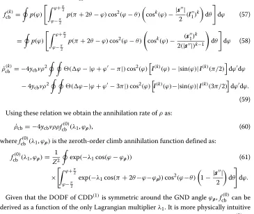
Given that the DODF of CDD(1)is symmetric around the GND angleϕρ,f_cb(0)can be derived as a function of the only Lagrangian multiplierλ1. It is more physically intuitive to express this rate as a function of the corresponding first dislocation momentM(1) = |ρ|/ρ, which can be understood as the GND fraction of the total dislocation density. As depicted in Fig. 9,f_cb(0)does not correspond to the parabolic rate expected by bimolecular annihilation of straight dislocation lines. The annihilation ofρcan be approximated by:

˙

ρcb= −1.2ycbvρρ

1−1.5

M(1) 2

+0.5

M(1)

6

. (62)

Similar to the CDD(1), the annihilation rate of the first three moment function of CDD(2)can be calculated using its DODF:

˙

ρ|cb=4ycbvρρf_cb(0)

M(1),M(2)

, (63)

˙

ρ(1)

1 _cb=4ycbvρfcb(1)

M(1),M(2)

=0, (64)

˙

ρ(2)

11 _cb=4ycbvρfcb(2)

M(1),M(2)

. (65)

Note that the first order annihilation function is always zero by definition

f_cb(1)=0

Fig. 9Blue line: climb annihilation function ofρas a function of the GND fraction. Green dashed-line: analytical fit (0.3(1−1.5x2+0.5x6)) to the annihilation rate. Red line: parabolic rate0.51−x2predicted by bimolecular annihilation

f_cb(0)M(1),M(2)≈

0.8M(2)−.52+0.3 1−M(1)2

, (66)

f_cb(2)M(1),M(2)≈0.5M(2)

1−M(1)2

. (67)

In the limit case ofM(2)=1, where dislocations become parallel straight lines, annihi-lation functions converge to parabolic bi-molecular annihiannihi-lation. The annihiannihi-lation rate of

ρ(2)_{can be evaluated using the relation between moment functions and alignment tensors} given by Monavari et al. (2016):

Fig. 10 Left column: the Zeroth and the second order annihilation functions as functions ofM(1)_andM(2)_.

˙

ρ(2) cb = ˙ρ

(2)

11 |cblρ⊗lρ+

˙

ρcb− ˙ρ₁₁(2)|cb

lρ⊥⊗lρ⊥ (68)

= −4ycbvρρ

f_cb(2)lρ⊗lρ+

f_cb(0)−f_cb(2)

lρ⊥⊗lρ⊥

.

Assuming an equi-convex microstructure where all dislocations have the same (mean) curvature, the annihilation rate of the total curvature density can be straightforwardly evaluated from the dislocation density annihilation rate:

˙

qcb= ˙ρcb q

ρ. (69)

The concomitant reduction in dislocation curvature density decreases the elongation (source) termvqin the evolution equation of the total dislocation density (10) – an effect which has an important long-term impact on the evolution of the dislocation microstruc-ture and may outweigh the direct effect of annihilation. The total annihilation rate is the sum of annihilation by cross slip and climb mechanisms.

Appendix 3

Cross slip annihilation in CDD(1)and CDD(2) Cross slip annihilation in CDD(1)

The cross slip annihilation rate of DODF in CDD(1)can be calculated by plugging the DODF of CDD(1)given by (50) into (28). Assuming that the dislocations have a smooth angular distribution which can be approximated as constant over the small angle interval 2ϕ, (28) can be further simplified:

˙

ρcs(ϕ)= −8ϕycsvρ(ϕ)ρ(π−ϕ)cos2(ϕ)(1− |sin(ϕ)|) = −8ϕycsvρρ

Z2exp(−λ1cos(ϕ−ϕρ)−λ1cos(π−(ϕ−ϕρ)))cos 2_(ϕ)(

1− |sin(ϕ)|)

(70)

The annihilation rate of the zeroth order alignment tensor (total dislocation density) is given by integrating (70) over all orientations:

˙

ρcs= −8ϕycsvρρ

1

Z2

exp(−λ1cos(ϕ−ϕρ)−λ1cos(π−(ϕ−ϕρ)))cos2(ϕ)(1− |sin(ϕ)|)dϕ

= −8ϕvycsρρfcs0.

(71)

f_cs0 is a function of the symmetry angle of DODF ϕρ and the Lagrangian multiplier λ1 or the correspondingM(1). We are especially interested in limit cases where the DODF is symmetric around the screw orientation and edge orientation which correspond to the axes of Fig. 12 (right). In the first case the GND vector is aligned with the screw orientationsϕρ = 0 andϕρ = πsuch thatρ(ϕ)=ρ(−ϕ)andM(1) =ρ1/ρ. Hence (71) becomes:

˙

ρcs= −4ycsv(ρ)2

2ϕ

Z2 cos

2_{(ϕ)(1− |sin(ϕ)|)dϕ}

ycsv

= −4ycsv(ρ)2

2ϕ

Z2

π− 4 3

, (72)

whereZ2is a function of the first momentM(1).

Fig. 11 Normalized annihilation rate as a function of the GND fractionM(1)_{for a dislocation annihilation}

triggered by cross slip. Blue line: normalized annihilation rate for a DODF symmetric around screw orientation (ϕ_ρ=0,π). Red line: normalized annihilation rate for a DODF symmetric around edge orientation

ϕρ=π2,

3π

2

. Dashed lines: Parabolic annihilation rate expected from the kinetic theory

˙

ρcs= −4ycsv(ρ)2

2ϕ

Z2 exp(−2λ1sin(ϕ))cos

2_{(ϕ)(1− |sin(ϕ)|)dϕ}

. (73)

For a completely isotropic dislocation arrangement,λ1 =0 andZ = 2π, we obtain in both cases:

˙

ρcs= −4ycsv(ρ)2

2ϕ

4π2 π−

4 3

. (74)

Figure 11 compares these two limit cases with the parabolic dependency expected according to kinetic theory for a system of straight parallel dislocations (dashed red line). In general, the annihilation rate can be approximated by interpolating between these two cases. Figure 12 shows the annihilation rate, normalized by the value atM(1) = 0, as a function of the GND fractionM(1) and the GND angleϕρ or the corresponding screw

and edge components of the normalized GND vectorρ/ρ. We can see that the

annihi-lation rate decreases monotonically with increasing GND fraction and goes to zero if all dislocations are GND.

Fig. 12 Left: cross slip annihilation functionfannof total dislocation density in CDD(1)plotted in polar

coordinates with the first dislocation momentM(1)_{as distance to the origin and the GND angleϕ}

ρ. The equivalent Cartesian coordinates are the screw and edge components of the normalized GND vector

ρ(1)_{=ρ/ρ. Middle: analytical approximation of the annihilation ratefcs=(ρ1)}2_cos2π|ρ| 2ρ

+(ρ2)2

1₋|ρ_ρ|2