Modeling in Earth system science up to and beyond IPCC AR5

R E V I E W

Open Access

Modeling in Earth system science up to and

beyond IPCC AR5

Tomohiro Hajima

, Michio Kawamiya

, Michio Watanabe

, Etsushi Kato

, Kaoru Tachiiri

, Masahiro Sugiyama

,

Shingo Watanabe

, Hideki Okajima

and Akinori Ito

Abstract

Changes in the natural environment that are the result of human activities are becoming evident. Since these changes are interrelated and can not be investigated without interdisciplinary collaboration between scientific fields, Earth system science (ESS) is required to provide a framework for recognizing anew the Earth system as one composed of its interacting subsystems. The concept of ESS has been partially realized by Earth system models (ESMs). In this paper, we focus on modeling in ESS, review related findings mainly from the latest assessment report of the Intergovernmental Panel on Climate Change, and introduce tasks under discussion for the next phases of the following areas of science: the global nitrogen cycle, ocean acidification, land-use and land-cover change, ESMs of intermediate complexity, climate geoengineering, ocean CO2uptake, and deposition of bioavailable iron in marine ecosystems. Since responding to global change is a pressing mission in Earth science, modeling will continue to contribute to the cooperative growth of diversifying disciplines and expanding ESS, because modeling connects traditional disciplines through explicit interaction between them.

Keywords:Earth system science; Earth system model; Carbon and nitrogen cycle; Land and ocean CO2uptake; Ocean acidification; Land-use and land-cover change; EMICs; Geoengineering; Iron deposition

Review

Introduction

Changes in the natural environment that are a result of human activities are becoming evident. Although one of the clearest examples is global warming, the problem goes well beyond a single issue and includes ocean acidification and perturbations of the global nitrogen cycle from indus-trial fixation. These issues are interrelated, and no single one can be addressed without interdisciplinary collabor-ation between scientific fields such as meteorology, ocean-ography, geochemistry, biology, and even social sciences. Recognizing the situation, scientists have been debating the necessity of ‘Earth system science’(ESS), in which the global environment is recognized as a system composed of its interacting subsystems - the atmosphere, oceans, bio-sphere, cryobio-sphere, and society.

Based on preceding studies on the concept of ESS, a report by the NASA Advisory Council (1988) first used the term‘Earth system science’explicitly and provided the clear definition used today. The report set the goal of ESS as the scientific understanding of the entire Earth system on a global scale by describing how its component parts and their interactions have evolved, how they function, and how they may be expected to continue to evolve on all time scales. The report points out that accomplishing this goal will require various research schemes such as nu-merical modeling, global observation systems, and infor-mation networks that enable efficient dissemination of observed data and research outputs. The statements made showed surprising foresight considering that at the time of publication, the use of the Internet was limited to certain advanced institutes and there were very few attempts to incorporate biogeochemical processes into general circula-tion models (GCMs).

Models used in Earth system science

As the aforementioned report emphasized, modeling can be a powerful tool for investigating the dynamics of the

* Correspondence:[email protected]

1_{Yokohama Institute for Earth Sciences, Japan Agency for Marine-Earth} Science and Technology, 3173-25 Showa-machi, Kanazawa-ku, Yokohama 236-0001, Japan

Full list of author information is available at the end of the article

Earth system. Models that have been developed and applied for this purpose can be categorized by their degree of complexity and integration. Models in the‘conceptual’ category, which are the least complex, consist of several simple equations mimicking certain aspects of complex behaviors of the Earth system (e.g., Budyko 1969; Sellers 1969). The degree of abstraction is, however, extremely high for this type of model, and correspondence between model equations and processes in nature is not readily understood. This leads to a fundamental difficulty in esti-mating model parameter values. Models in this category are therefore mainly used for educational purposes or as supporting material for constructing a theoretical frame-work and are rarely used for projection.

In contrast, atmospheric and oceanic GCMs have been applied to the projection of El Niño events, global warming, and others. GCM-based Earth system models (ESMs), which are introduced in the next section, have a drawback in that they are computationally expensive. To fill the gap between conceptual models and GCMs, ESMs of intermediate complexity (EMICs) are now be-ing extensively developed (Claussen et al. 2002). EMICs greatly simplify equations of motion for the atmosphere and ocean and radiation processes, retaining some abil-ity to reproduce realistic properties such as geographic temperature distribution and deep water formation. EMICs require much less in terms of computer re-sources and can be integrated for many thousands of years without supercomputers.

With careful experiment design, EMICs constitute an important element for future projection and interpret-ation of past events with time scales longer than approximately a few hundred years (e.g., Timmermann

et al. 2009; Hargreaves et al. 2012). However, the same drawback of substantial abstraction for conceptual models applies to EMICs, albeit to a lesser extent. It is desirable to make parallel and complementary use of GCM-based ESMs and EMICs within computer resource availability.

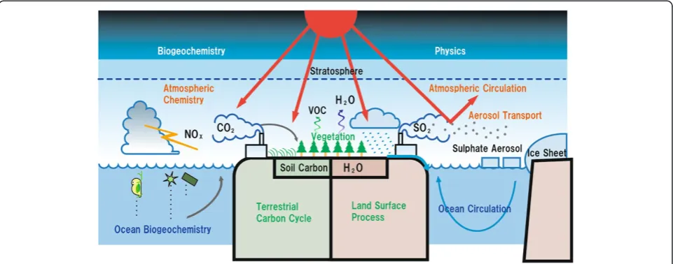
Many institutes in the world involved in global warm-ing projection are developwarm-ing elaborate ESMs by coup-ling biogeochemical modules (vegetation dynamics, the carbon cycle, and others) with GCMs (Figure 1). This figure shows components specific to the Model for Interdisciplinary Research on Climate, Earth System Model (MIROC-ESM; Watanabe et al. 2011). This is a GCM-based ESM developed by the Japan Agency for Marine-Earth Science and Technology (JAMSTEC), with collaboration from The University of Tokyo Atmosphere Ocean Research Institute (AORI) and National Institute for Environmental Studies (NIES). Most ESMs devel-oped by leading institutes have similar structures. One of the most striking findings from studies using ESMs is that there is positive feedback between climate change and the carbon cycle (IPCC 2013), mainly caused by re-sponse of the terrestrial biosphere to rising temperature.

For coupling the carbon cycle to climate models, a new method of climate-carbon cycle simulation has been devised and adopted as a common method of climate-carbon cycle projection. Traditionally, ESMs are driven by ‘CO2 emission’, in which future climate

change is projected by internally predicted CO2

con-centration based on prescribed anthropogenic CO2

emission (e.g., Friedlingstein et al. 2006; Yoshikawa et al. 2008; Friedlingstein et al. 2014). This type of simulation reflects the actual sequence of the global carbon cycle and is therefore very intuitive. However, it is difficult to

effectively compare ESM results with other conven-tional GCMs, because different CO2concentrations are

referenced in these two types of climate model.

Alternatively, in the new method, with so-called‘ concen-tration-driven’ simulations, the rates of the atmosphere-ocean and atmosphere-land CO2exchanges are diagnosed

in ESMs by referring to the prescribed CO2

concentra-tion and predicted climate. Because uncertainty arising from carbon cycle processes can be excluded in the projected climate, we can effectively compare climate-related variables (such as temperature and climate sen-sitivities) between ESMs and GCMs (e.g., Andrews et al. 2012; Knutti et al. 2013). Another feature of this concentration-driven method is that by using the pre-scribed CO2 concentration and diagnosed CO2 fluxes,

we can inversely estimate the anthropogenic CO2

emis-sion that is allowed to achieve the prescribed CO2

concen-tration pathways. Since the rate of emission is almost equivalent to that of anthropogenic fossil fuel CO2, this

in-versely estimated CO2 emission in the experiments is

sometimes called‘allowable’or‘compatible’emission. For example, in the study of Jones et al. (2013), compatible emissions simulated by ESMs were compared by applying prescribed CO2pathways of representative concentration

pathways (RCPs). These authors found that about half the participating models predicted that ‘negative’ anthropo-genic emissions will be necessary during the twenty-first century to realize RCP2.6 scenarios. As such information from the concentration-driven experiments has a direct implication for future climate mitigation policies, this simulation style is now becoming popular among those who use ESMs, suggesting a new application of models in ESS for global environmental change projections.

Future directions

It has been pointed out that the behavior of the simulated terrestrial biosphere may be drastically changed if one in-cludes the nitrogen cycle. The intensity of climate-carbon cycle feedback based on models with a global nitrogen cycle will be an issue of great interest for the possible next phase of the Intergovernmental Panel on Climate Change (IPCC) assessment, as explained in the ‘Nitrogen cycle’ section.

Although the ocean exhibits feedback caused by the temperature dependence of the CO2 solubility in

seawater, its intensity is about a quarter of that of the terrestrial biosphere, at least under the current setup of typical ESMs, often without a terrestrial nitrogen cycle (IPCC 2013). The projection of the ocean uptake of CO2

is nevertheless critical, because the ocean will be the pri-mary sink of anthropogenic CO2(details in‘Ocean CO2

uptake’section) and the uptake causes another problem, ocean acidification caused by the weak acidity of CO2.

The ocean acidification problem is reviewed in more detail in the‘Ocean acidification’section.

It is sometimes purported that the role of global envir-onmental projection is gradually changing from science used as a warning to that which can be implemented (Kerr 2011). Indeed,‘actionable science’ was the watch-word in the 2011 Open Science Conference of the World Climate Research Programme (WCRP) in Denver (Asrar et al. 2012). Climate models can serve society in many ways, such as providing information on extreme weather. ESMs are particularly useful for reflecting scien-tific perceptions of future socioeconomic scenarios. Com-ponents of ESMs for global cycles of carbon and other biogeochemical properties can act as a bridge between so-cioeconomic models, whose outputs are frequently green-house gas emissions, and climate models, which require concentrations of the gases. Another aspect of the way in which ESMs are helpful for linking climate science and the socioeconomy is that they can deal with land-use change (LUC) processes, a key factor for the future global carbon budget and regional climate change. Issues of LUC are surveyed in the ‘Land-use and land-cover change’ section. Care must be taken regarding uncertainties when ESM results are applied to developing socioeconomic scenarios. Uncertainties in parameter values of ESMs are even more serious than those in conventional climate models, because ESMs incorporate biological processes such as photosynthesis. Parameter ensemble experiments are desirable but not always feasible, owing to the compu-tational cost of GCM-based ESMs. Using GCM-based ESMs and EMICs in parallel may remedy this problem, as discussed in the section titled ‘Earth system models of intermediate complexity’.

Actionable science might go well beyond just providing information. Artificial, active modification of the global climate, often termed geoengineering, is now a matter of debate. The Fifth Assessment Report (AR5) of IPCC (IPCC 2013) treated this issue in multiple chapters. This should, however, be regarded as a last resort since most of its side effects are yet to be assessed and there will un-doubtedly be many others of which we are not yet aware. Scientists have started a project to evaluate the effects of geoengineering using numerical models. Results from that project will be introduced in the section titled ‘Climate geoengineering,’together with other aspects of geoengi-neering presented in the ‘Ocean CO2 uptake’ and

‘Atmospheric deposition of bioavailable iron in marine ecosystems’sections.

enhancing the credibility of future projection, since paleoclimate provides the only means for validating cli-mate models on time scales longer than decades. A lim-ited number of topics are addressed in this review, from an extremely large number of fields in which ESMs can be applied.

Nitrogen cycle

Modern Earth system modeling may be said to have begun by incorporating land/ocean carbon cycle processes into GCMs (Cox et al. 2000). The latest ESMs are now equipped with more complex and interactive processes on global chemical/biogeochemical processes, such as atmos-pheric chemistry. Recent studies analyzing simulation results from the Coupled Model Intercomparison Project phase 5 (CMIP5) ESMs suggest the importance of the glo-bal nitrogen cycle, particularly the process of nitrogen shortage and its limitation on ecosystem productivity (Arora et al. 2013; Hajima et al. 2014). This deficiency of available nitrogen could alter the behavior of the global carbon cycle, thereby impacting the global climate. In addition, from the beginning of the twentieth century, the global nitrogen cycle has been greatly perturbed by the human creation of reactive nitrogen and anthropogenic emission of large amounts of N2O, one of the strongest

greenhouse gases (Gruber and Galloway 2008). To quan-tify historical human effects on the global nitrogen cycle and make projections for future climate change, ESMs with an explicit nitrogen cycle can be a powerful tool. Here, we first summarize the interaction of climate and the carbon cycle and then describe the impacts of the glo-bal nitrogen cycle on the climate by regulating the gloglo-bal carbon budget. Finally, the direct impacts of the nitrogen cycle on the climate due to the production of greenhouse and associated gases are briefly summarized.

Feedback on carbon cycle from environmental changes

The global carbon cycle has long been regarded as one of the major components that control the global climate because CO2in the atmosphere has a greenhouse effect

and its concentration is regulated by ocean and land ecosystems through the exchange of CO2 with the

at-mosphere. Furthermore, human activities such as fossil fuel combustion, land-use change, and cement produc-tion have released large amounts of CO2into the air. Its

concentration is now reaching 400 ppmv, which corre-sponds to about a 40 % increase from the preindustrial state. Changes of global carbon balance in the industrial era can be simply understood by

FF¼ΔCAþΔCLþΔCO; ð1Þ

where FF is the cumulative amount of carbon emitted by fossil fuel combustion andΔCrepresents the changes in

the carbon amounts from the preindustrial state of the atmosphere (A), ocean (O), and land (L). In this formu-lation, the partitioning of emitted carbon between the atmosphere, ocean, and land ecosystems is variable; envir-onmental changes such as global warming can change the capability of carbon uptake by land and the ocean and thereby alter the airborne fraction of emitted CO2

(Le Quéré et al. 2013; Jones et al. 2013 for treatment of land-use change effects on the global carbon balance). For example, global warming could induce large ecosys-tem respiration and thus reduce total terrestrial carbon. To understand such interactive behavior of the carbon cycle and climate, Friedlingstein et al. (2003) proposed a simple mathematical expression to link carbon balance and environmental changes:

ΔCL;O¼βL;OΔCAþγL;OΔT ð2Þ

The first term on the right represents a change in the amount of stored carbon due to an atmospheric CO2

increase, assuming a linear response of carbon storage to increasing atmospheric CO2(ΔCA) with coefficientβ.

This environmental effect on carbon storage is sometimes called ‘CO2-carbon feedback’. Because an increased CO2

concentration promotes carbon uptake by land and oceans (by stimulating photosynthesis in land ecosystems and increasing the CO2 partial pressure deficit between

the atmosphere and oceans), β is considered to have a positive sign (i.e., CO2-carbon feedback is negative) (Arora

et al. 2013; Friedlingstein et al. 2006; Gregory et al. 2009). The second term represents a carbon storage change in response to climate change (represented byΔT, the degree of warming); this process is called ‘climate-carbon feed-back’. Since warming could cause larger ecosystem respir-ation and a reduction of CO2 dissolution in water, the

feedback parameter γis regarded to have a negative sign (Arora et al. 2013; Friedlingstein et al. 2006; Gregory et al. 2009), meaning that interaction between climate and the carbon cycle forms a positive feedback loop.

By combining these two equations, we obtain an expression that incorporates environmental change (ΔCAandΔT) into the global carbon balance:

FF¼ΔCAþβL;OΔCAþγL;OΔT ð3Þ

This equation indicates that cumulative carbon con-tained in fossil fuel emission increases atmospheric carbon (ΔCA), but carbon partitioning in the atmosphere depends

on the land/ocean carbon cycle response, CO2-carbon

(βΔCA) and climate-carbon (γΔT) feedbacks. A recent

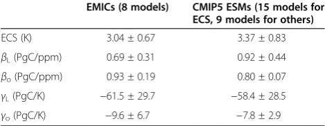
study by Arora et al. (2013) in CMIP5 compared these feedback strengths for nine ESMs via sensitivity analysis (Table 1), showing that land and ocean carbon cycles have comparable levels of CO2-carbon feedback. As

for the ocean. The climate-carbon feedback for land was greater (negative) than that for the ocean, at−58.4 and −7.8 PgC K−1 respectively. In their simulations, although the CO2growth rate was rapid (CO2increase

of 1.0% year−1during 140 simulation years) and thus sub-stantial global warming was expected, most ESMs showed that CO2-carbon feedback surpassed climate-carbon

feed-back across all simulation periods, so natural carbon sinks continued to absorb anthropogenic carbon in the simulations.

Nitrogen cycle feedback on carbon cycle

The global nitrogen cycle is one of the most important biogeochemical cycles, together with that for carbon. Al-though the total mass flux of global nitrogen is much smaller than that of carbon (Gruber and Galloway 2008), the nitrogen cycle may have strong impacts on the car-bon cycle. Since nitrogen is used by organisms to make amino acids, enzymes, proteins, and nucleic acids, the nitrogen cycle in ecosystems is intimately associated with the life functions of organisms. It is used to develop organisms' bodies, maintain their activity, and increase their populations (Canfield et al. 2010). However, since most nitrogen in nature is in an inactive form (N2),

nitrogen in reactive and available forms for ecosystems (such as ammonia and nitrous oxide) may be rare and thus often be a limiting factor for ecosystem productiv-ity. This deficiency of nitrogen can strongly restrict carbon fluxes in ecosystems, hence having a feedback effect on the global climate.

In Equation 3, the nitrogen cycle feedback on the climate-carbon cycle system can be summarized as fol-lows. First, the amount of available nitrogen for plants and phytoplankton can control their productivity and the resultant carbon fluxes out of the atmosphere to land or ocean. As shown by free-air CO2enrichment studies,

an elevated CO2 concentration on land can stimulate

photosynthesis and accumulate biomass. However, if the amount of available nitrogen does not meet demands for plant growth, the plant biomass accumulation rate is

likely constrained (e.g., Reich et al. 2006; Reich and Hobbie 2013). For ocean ecosystems, the gross prod-uctivity of phytoplankton and its spatial distribution are originally and strongly regulated by the available nitro-gen amount, even in current conditions (Canfield et al. 2010). Because most terrestrial ecosystem models in ESMs are now incapable of explicitly representing the influence of a nitrogen deficit on photosynthetic cap-acity or other physiological aspects (e.g., leaf area), ni-trogen feedback should be reflected by the parameterβ to weaken the strength of negative CO2-carbon

feed-back. In fact, some CMIP5 ESMs incorporating explicit terrestrial nitrogen cycle processes show a weaker re-sponse to increasing CO2 than those output by other

models, which is likely due to the nitrogen-limited re-sponse of plant productivity in an enriched CO2world

(Arora et al. 2013; Hajima et al. 2014).

Furthermore, the nitrogen cycle on land could affect the carbon storage response to climate change, as repre-sented by parameterγin Equation 3. Since global warm-ing could lead to enhanced activities of soil microbes, accelerated soil decomposition may reduce the total amount of soil carbon. However, accompanied by the re-lease of inorganic nitrogen that becomes soil nutrients, this accelerated soil decomposition rate might activate plant productivity. In fact, some models incorporating explicit terrestrial nitrogen cycle processes reduce the carbon cycle response to global warming, with less nega-tive or sometimes slightly posinega-tive values for γ (Sokolov et al. 2008; Bonan and Levis 2010; Thornton et al. 2009; Zaehle et al. 2010). In these models, although global warming reduces soil carbon storage because of en-hanced heterotrophic respiration, increasing soil nutri-ents somewhat compensates the global terrestrial carbon reduction by increasing vegetation carbon storage.

The global nitrogen cycle could alter the global climate by changing both the CO2-carbon and climate-carbon

feedback, thereby creating climate-carbon-nitrogen in-teractions. Although the number of studies is limited, ESMs with a nitrogen cycle show a similar trend in that the incorporation of a nitrogen cycle reduces the sensi-tivity of the carbon cycle response to environmental changes. However, constraints of the nitrogen cycle on the carbon cycle should be addressed with the presence of reactive nitrogen in the atmosphere, as described below.

Direct impact of the nitrogen cycle on climate and human perturbations

In the previous section, we described nitrogen cycle feedbacks on the climate through the regulation of carbon cycle responses. In addition, the nitrogen cycle directly impacts global climate because the greenhouse gas N2O has a relatively long lifetime in the atmosphere,

Table 1 Equilibrium climate sensitivity (ECS), and concentration (β) and climate (γ) carbon cycle feedback strengths

EMICs (8 models) CMIP5 ESMs (15 models for ECS, 9 models for others)

ECS (K) 3.04 ± 0.67 3.37 ± 0.83

βL(PgC/ppm) 0.69 ± 0.31 0.92 ± 0.44

βo(PgC/ppm) 0.93 ± 0.19 0.80 ± 0.07

γL(PgC/K) −61.5 ± 29.7 −58.4 ± 28.5

γo(PgC/K) −9.6 ± 6.7 −7.8 ± 2.9

more than 100 years. Galloway et al. (2004) estimated the total N2O emission under conditions before the

significant human perturbation at approximately 12 TgN year−1. Its emission rate has greatly increased during the industrial era because human activities such as industrial nitrogen fixation for fertilizer, fossil fuel/biomass combus-tion, and agriculture have increased the total amount of reactive nitrogen globally (Galloway et al. 2004; Gruber and Galloway 2008). Some studies using data assimilation or inversion techniques established the current total global N2O emission at approximately 18 TgN year−1, and

the contribution of the anthropogenic emission to the glo-bal total at approximately one third (Saikawa et al. 2013 estimate for 2002 to 2005). The latter emission has in-creased its concentration in the atmosphere and thus N2O

radiative forcing is now considered to be 0.17 W m−2, about 10% of CO2radiative forcing (IPCC 2013).

Further-more, such human activities have created other forms of reactive nitrogen, namely, NOx, NHx, and NOy. Nitrogen in these reactive forms interacts with global and local cli-mates by contributing to the formation of aerosols, acting as a precursor for generating tropospheric ozone, and through its association with CH4reduction (Menon et al.

2007).

Reactive nitrogen in these forms may further affect carbon-nitrogen interactions. Since net radiative forcing of these agents is positive (IPCC 2013), there could be an additional warming that could accelerate soil decom-position and modify carbon cycle feedbacks on the climate. In addition, since inorganic mineral nitrogen could be an ecosystem resource for productivity, its de-position on land and ocean surfaces could also have in-direct impacts on the climate by alleviating the nitrogen limitation on productivity (e.g., Bonan and Levis 2010; Thornton et al. 2009). Although it is important to assess the combined effect of direct (changing atmospheric composition of non-CO2greenhouse gases) and indirect

(changing CO2 concentration via modulating carbon

cycle feedbacks) impacts of the nitrogen cycle on the global climate, the number of related studies is limited (e.g., Stocker et al. 2013; Zaehle et al. 2011). For compre-hensive understanding of the influence of human activity on the global nitrogen cycle and its propagation impacts on the global environment, it is hoped that more scien-tific efforts will be made using fully coupled carbon-nitrogen-climate models.

Ocean acidification

Definition of ocean acidification

The emission of large amounts of anthropogenic carbon dioxide has increased the global atmospheric CO2

concen-tration and contributes to temperature increases in the atmosphere and ocean. Since 1750, the global ocean has absorbed about a third of anthropogenic CO2 released

into the atmosphere (Sabine et al. 2004; Sabine and Feely 2007). CO2 reacts with water molecules (H2O) to form

the weak acid H2CO3 (carbonic acid), and most of this

acid dissociates into hydrogen ions (H+) and bicarbonate ions (HCO3−), such as

H2OþCO2↔H2CO3

H2CO3↔HþþHCO−3

Some of the resulting H+ reacts with carbonate ions CO32− to produce additional HCO3− ions.

HþþCO₃2−↔HCO−₃

As a result, CO2dissolution in the ocean increases H+

(thereby decreasing pH) and reduces CO32−

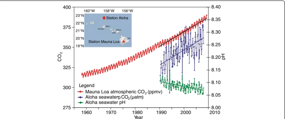
concentra-tions, a process known as ocean acidification (Broecker and Clark 2001; Caldeira and Wickett 2003, 2005; Doney et al. 2009). Figure 2 shows a time series of the atmos-pheric CO2 at Mauna Loa as well as the surface ocean

CO2partial pressure (pCO2) and surface ocean pH at the

ocean station ALOHA in the subtropical North Pacific Ocean. We see that as atmospheric CO2rises, some extra

CO2 is transferred into ocean surface waters, leading to

ocean acidification. The pH of ocean surface waters has decreased by about 0.1 since the dawn of the industrial era (Caldeira and Wickett 2003, 2005), with a decrease of approximately 0.0018 year−1observed over the last quarter century at several open-ocean time-series sites (Bates 2007; Bates and Peters 2007; Santana-Casiano et al. 2007; Dore et al. 2009).

Marine calcifying organisms such as plankton, shellfish, coral, and fish use carbonate ions CO32− to build their

shells or skeletons from calcium carbonate (CaCO3),

Ca2þþCO₃2−↔CaCO3;

so they are expected to be greatly affected by ocean acidifi-cation. The carbonate ion concentration is often expressed by the degree of saturation of biominerals aragonite (ΩAr)

and calcite (ΩCa) (Feely et al. 2004). Shell and skeleton

for-mation generally occurs in supersaturated sea waterΩ> 1 and dissolution in undersaturated seawaterΩ< 1. Conse-quently, spatial and temporal changes in saturation state with respect to these mineral phases are important for understanding how ocean acidification might substantially impact future ecosystems.

Assessment by ESMs

We can assess the ocean's present and future ability to take up anthropogenic CO2 and the influence of ocean

during the twenty-first century, across all the world's oceans. By the middle of the present century, atmospheric CO2 levels could reach more than 500 ppm and exceed

800 ppm by the end of the century (Friedlingstein et al. 2006, 2014). By 2100, these CO2levels would result in an

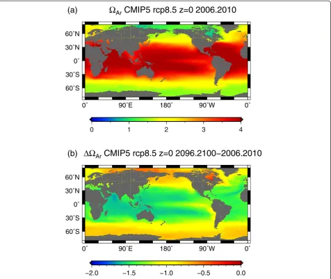
additional decrease of surface water pH by 0.3 units over current conditions and 0.4 over the preindustrial level. This represents an increase in the ocean's hydrogen ion concentration H+ by 2.5 times relative to the beginning of the industrial era (Orr et al. 2005; Feely et al. 2009). Figure 3 shows the multi-model mean aragonite satur-ation state averaged over 2006 to 2010 and 2096 to 2100, under a scenario called a RCP (http://www.pik-potsdam. de/~mmalte/rcps/) in AR5. Although the greatest decline of surface CO32−occurs in the warmer low and middle

lati-tudes (Feely et al. 2009) whereΩAr> 3 (Figure 3a,b), it is

lowΩArwaters at high latitudes and in upwelling regions

that first become undersaturated with respect to aragonite. ESMs show that this aragonite undersaturation in surface waters is reached before the end of the twenty-first cen-tury in the Southern Ocean (Orr et al. 2005). Steinacher et al. (2009) suggested that aragonite undersaturation occurs sooner and is more intense in the Arctic. When atmospheric CO2reaches 428 ppm, 10% of Arctic surface

waters are projected to become undersaturated. By 2100, atmospheric CO2will exceed 800 ppm and much of the

Arctic surface is projected to become undersaturated with respect to calcite (Feely et al. 2009). This means that sur-face waters would be corrosive to all CaCO3minerals.

These changes extend well below the sea surface (Orr et al. 2005). Throughout the Southern Ocean, the entire water column becomes undersaturated with respect to

aragonite. During the twenty-first century, the aragon-ite saturation horizon, representing the limit between undersaturation and supersaturation in the Southern Ocean and subarctic Pacific, shoals to the sea surface. In the North Atlantic, surface waters remain saturated with respect to aragonite, but the aragonite saturation horizon shoals dramatically, e.g., north of 50°N it shoals from 2,600 to 115 m. Greater erosion in the North Atlantic is due to deeper penetration of waters with higher con-centrations of anthropogenic CO2from the sea surface

(Sarmiento et al. 1992; Gruber 1998; Sabine et al. 2004). Surface CaCO3 saturation also varies seasonally,

par-ticularly at high latitudes, where observed saturation is higher in summer and lower in winter (Merico et al. 2006; Findlay et al. 2008). Future projections using ocean carbon cycle models indicate that undersaturated condi-tions will be reached first in winter (Orr et al. 2005). In the Southern Ocean, it is projected that wintertime under-saturation with respect to aragonite will begin when at-mospheric CO2reaches 450 ppm, which is about 100 ppm

sooner (30 years) than for the annual mean ation (McNeil and Matear 2008). Aragonite undersatur-ation will be reached during wintertime in parts (10%) of the Arctic when atmospheric CO2 attains 410 ppm

(Steinacher et al. 2009).

Controlling factors

As mentioned above, future reductions in surface ocean pH and CaCO3 (calcite and aragonite) saturation states

are mostly controlled by the uptake of anthropogenic CO2. Other effects of future climate change counteract

less than 10% of the reductions of CaCO3 saturation

400

375

350

325

300

275

CO

2

8.40

8.35

8.30

8.25

8.20

8.15

8.10

8.05

8.00

pH

1960 1970 1980 1990 2000 2010 Mauna Loa atmospheric CO2(ppmv)

Aloha seawaterpCO2(µatm)

Aloha seawater pH Legend

160°W 158°W 156°W 23°N

22°N

21°N

20°N

19°N

Station Mauna Loa Station Aloha

Honolulu Kailua

Kihei Kahului

Hilo

Year

Figure 2Observed partial CO2pressure (pCO2) and ocean pH at ocean surface. pCO2(μatm; blue) and surface ocean pH (green) at

ocean are observed at Station ALOHA in subtropical North Pacific Ocean, in comparison with atmospheric CO2concentration observed

at Mauna Loa (in parts per million by volume; red).Note that the increase in oceanic CO2over the past 17 years is consistent with the

(Orr et al. 2005; McNeil and Matear 2008). An exception is the Arctic Ocean, where decreases in the pH and aragonite saturation state are predicted to be caused by increased freshwater input from sea ice melt, enhanced precipitation, and stronger air-sea CO2fluxes because of

less sea ice cover (Steinacher et al. 2009; Yamamoto et al. 2012). This result indicates that future projections of the pH and aragonite saturation state at high latitudes may be significantly influenced by rapid sea ice reduction as well as increases of atmospheric CO2concentration.

Focusing on the regional ocean carbon cycle, models project some nearshore systems to be highly vulnerable to future pH decrease. In the California Current system, an eastern upwelling system, strong seasonal upwelling of carbon-rich waters (Feely et al. 2008) makes surface waters sensitive to future ocean acidification, as in the Southern Ocean. In the northwestern European shelf seas,

large spatiotemporal pH variability is enhanced by local effects from river input and organic matter degradation, exacerbating ocean acidification from anthropogenic CO2

invasion (Artioli et al. 2012). In the Gulf of Mexico and East China Sea, coastal eutrophication, another anthropo-genic perturbation, has been shown to enhance subsurface acidification as additional respired carbon accumulates at depth (Cai et al. 2011).

Land-use and land-cover change

On the land surface, about one-third to one-half the area of natural ecosystems has been converted to managed land for use as cropland and pasture over the past 10,000 years (Klein Goldewijk et al. 2011). Human land use is projected to expand in the future because of food and energy demands due to changes in the population and socioeconomic factors (Bruinsma 2009). Anthropogenic

(b)

ΔΩ

CMIP5 rcp8.5 z=0 2096.2100−2006.2010

0˚ 90˚E 180˚ 90˚W 0˚ 60˚S

30˚S 0˚ 30˚N 60˚N

−2.0 −1.5 −1.0 −0.5 0.0

(a)

Ω

CMIP5 rcp8.5 z=0 2006.2010

0˚ 90˚E 180˚ 90˚W 0˚ 60˚S

30˚S 0˚ 30˚N 60˚N

Figure 3Spatial distribution of aragonite saturation state_ΩAr. (a)Model-meanΩArat the sea surface averaged over 2006 to 2010, derived

modification of land cover and its management affect ecosystem functioning and also modifies Earth system atmosphere-biosphere interactions through biogeophy-sical and biogeochemical effects (Claussen et al. 2001; Pongratz et al. 2010; Sato et al. 2014). Changes in surface albedo and latent and sensitive heat fluxes are principal biogeophysical effects of use and land-cover changes, which affect atmospheric conditions via changes to the hydrologic cycle and energy balance (Bonan 2008). A striking example of the biogeophysical effect of land-use change is that of historical deforest-ation at mid and high latitudes, which has increased surface albedo in winter by altering snow cover and lowering surface air temperature (Davin and de Noblet-Ducoudré 2010). In the tropics, deforestation reduces evapotranspiration, which also affects atmospheric con-ditions (Bala et al. 2007). Furthermore, irrigation and soil management on cropland is known to affect local air temperatures (Lobell et al. 2006).

The dominant biogeochemical effect of historical land-use and land-cover change is an increase in the atmos-pheric CO2concentration, through decreases in terrestrial

carbon stock via expansion of anthropogenic land use (Sato et al. 2014). About 33% of total anthropogenic CO2

emissions from the preindustrial era are from land-use change (Houghton et al. 2012). It is also pointed out in several studies (Bouwman et al. 2005; Bodirsky et al. 2012) that increases in atmospheric N2O, for which the

global-warming potential over 100 years is about 300 times that of CO2, are caused by emissions from the increased use of

fertilizer on cropland.

For a quantitative understanding of the biogeophysical and biogeochemical effects of land-use and land-cover change, model intercomparison was first done using EMICs. These couple terrestrial biogeochemical models with simplified lower-resolution climate models (Brovkin et al. 2006) and then GCMs with land surface schemes, with consideration of anthropogenic land-cover type (Pitman et al. 2009). To incorporate changes of land-cover type, anthropogenic land use as a fraction of each land-use type for a grid cell in forcing data is assigned annually in the model. To represent biophysical proper-ties of anthropogenic land-use type such as cropland, pasture, and urban (if considered in the land-use data), each plant functional type that has corresponding land surface scheme parameters (such as phenological, mor-phological, and photosynthetic) is allocated a percentage at a grid cell annually, according to land-use forcing data. Effects on the carbon budget caused by land-cover and land-use change are estimated through carbon emis-sions from deforestation and wood harvesting. This esti-mation is done using several product pools with various time scales of decay (McGuire et al. 2001) and additional carbon uptake after the abandonment of cropland by

vegetation regrowth, which can be affected by the age distribution of vegetation on secondary land (Shevliakova et al. 2009).

Pongratz et al. (2010) evaluated the effect of land-use change throughout the twentieth century using a GCM-based ESM. They estimated the effect of land-use change on the global mean temperature in the twentieth century to be −0.03°C through biogeophysical effects and 0.18°C through biogeochemical effects, giving a net effect of 0.15°C. Generally, biogeophysical effects of historical land-use change on the global mean surface air temperature are less than biogeochemical effects, because the former operates locally and biogeophysical changes from deforest-ation (e.g., those of albedo and latent heat flux) sometimes work together to compensate their individual impacts on temperature (Pitman et al. 2009; Pongratz et al. 2010).

Uncertainty of land-use and land-cover change

In such evaluations of impacts on the atmosphere by glo-bal land-use change, large uncertainties persist among model estimates (Sato et al. 2014). For example, in the study of the current global carbon budget, one of the lar-gest uncertainties originates from anthropogenic land-use changes in terrestrial ecosystems. The standard deviation of carbon flux caused by historical anthropogenic land-use change is estimated to be in the order of ±0.5 PgC (Le Quéré et al. 2013). The choice of land-use data could be one of the causes of estimate variations in land-use change emissions (Jain and Yang 2005; Meiyappan and Jain 2012). In the global evaluation of use and land-use change effects, land-land-use data compiled at an approxi-mately 0.5° × 0.5° spatial resolution are generally used. Uncertainty in gridded historical land-use data derives from differences in cropland and pasture area between datasets, downscaling processes of regionally aggregated data, and others. These uncertainties in the reconstruction of historical land-use data should be considered in model evaluation (Klein Goldewijk and Verburg 2013). In a re-cent study of the global carbon budget, the standard devi-ation of estimated land-use change flux with multiple terrestrial carbon cycle models using the same land-use dataset was estimated at 0.42 PgC year−1(Le Quéré et al. 2013). In contrast, the standard deviation estimated by a single model, which was also used in the multiple model comparison using three different land-use datasets, was 0.27 PgC year−1(Jain et al. 2013).

these. These include differences in the implementation of land-use data in the terrestrial ecosystem component among models, and whether the model considers emis-sions and uptake caused by shifting cultivation, wood harvesting, forest degradation, crop harvesting, peat fires, and others.

LUC in CMIP5 and its future direction

In CMIP5, anthropogenic land-use and land-use changes were considered in historical and future scenarios simu-lated by ESMs. Harmonized land-use transition datasets have been prepared through historical (1500 to 2005) and four future RCPs through 2100 (Hurtt et al. 2011). The historical part consists of the reconstructed crop-land and pasture dataset‘History Database of the Global Environment’(HYDE) (Klein Goldewijk et al. 2010; Klein Goldewijk et al. 2011) and wood harvest data of the Food and Agriculture Organization (FAO) of the United Nations. Four future scenarios constructed by integrated assessment models (IAMs) were harmonized with the historical data to smoothly connect past and future sce-narios in 2005, using consistent land-use categories. These are primary land, secondary land, cropland, pasture, and urban areas, with a 0.5° × 0.5° horizontal resolution. An-nual transitions among these land-use categories, wood harvest area, and carbon mass changes were calculated for each grid cell. In the CMIP5 experiments, ESM modelers used harmonized land-use data as common forcing to consider the effects of land-use change on the terrestrial carbon cycle and biogeophysical effects of land-cover change in climate simulations (Taylor et al. 2012). In addition to the standard CMIP5 experiments, the inter-national project Land-Use and Climate, Identification of Robust Impacts (LUCID) conducted LUCID-CMIP5 ex-periments using ESMs, in which land use was fixed at 2005 to evaluate future land-use scenarios (Brovkin et al. 2013). Under the LUCID framework, biogeophysical effects and variation of the carbon cycle from future land-use change was evaluated using concentration-driven simulations of RCP2.6 and RCP8.5 (Brovkin et al. 2013; Boysen et al. 2014). In this simulation, there were no significant impacts on the global climate from biogeo-physical changes caused by future land-use change. How-ever, in regions exceeding 10% land-use change during the scenario period, half the models showed significant im-pacts of such change on surface temperature. Further-more, some models revealed significant changes in surface albedo, latent heat flux, and available energy in the 10% exceedance region. Nevertheless, these biogeophysical ef-fects on climate in the future scenarios were weak because the area of intense land-use change was restricted to trop-ical and subtroptrop-ical regions and the changed area was small compared with historical changes. For effects on terrestrial carbon storage, all models showed significant

decreases in carbon stock in the two RCP scenarios. Esti-mations of cumulative carbon emission caused by land-use change varied greatly among the models, suggesting scientific issues in implementing land-use change pro-cesses in the ESMs (e.g., some models considered both crop and pasture areas, whereas others treated only crop-land; some models used information on gross land-use transitions, whereas others used net transitions).

After the CMIP5 exercise, needs were recognized for more detailed protocols to handle anthropogenic land use and land-use change in land surface models. Consider-ation of more precise land-use categories and management processes such as irrigation, wood harvest treatment, bio-fuel crop type, and afforestation have been addressed for the upcoming 6th phase of Coupled Model Intercompari-son Project (CMIP6). This is because the future carbon cycle is strongly dependent on the land-use scenario as well as the terrestrial ecosystem response to both future CO2 and climate change (Jones et al. 2013). Toward

CMIP6, experiments involving land-use are also consid-ered in specialized intercomparisons that would use CMIP6 standards and infrastructure. In this process, especially for future scenario simulations, the validation of simulated carbon stock in contemporary land ecosys-tems would be of great importance, because bias in CMIP5 historical simulations is one cause of strong variability in the simulated future changes of carbon stock within CMIP5 and LUCID-CMIP5 simulations (Brovkin et al. 2013; Anav et al. 2013). In addition, C-N interaction for CO2 fertilization effects should be

con-sidered because of their strong impacts on vegetation regrowth following land-use change, which in turn affects contemporary and future terrestrial carbon sink trends (Jain et al. 2013).

Earth system models of intermediate complexity

State-of-the-art GCMs/ESMs furnish irreplaceable future projection data. These models are designed to maximize the representation of detailed processes while retaining reasonable computational speed so that experiments are completed as scheduled, and are unsuitable for executing very long runs or ensemble experiments sufficiently large to extract statistically useful information. In contrast, sim-ple box models aid conceptual understanding, but a lack of geographic detail prevents practical applications and their implications are more qualitative than quantitative. EMICs are designed to fill the gap between the two model types. EMIC results are sometimes included in inter-model comparisons of ESMs, e.g., the Coupled Climate Carbon Cycle Model Intercomparison Project (C4MIP) (Friedlingstein et al. 2006), which shows results compar-able to ESMs.

(1980). More than ten models developed prior to Claussen et al. (2002) defined the term EMICs based on three fac-tors: the number of interacting components of the climate system explicitly represented in the model, the number of processes explicitly simulated, and the detail of descrip-tion. The number of models increased to 13 by the time EMICs were summarized by Claussen (2005). As de-scribed below, we had 15 models in the latest EMIC model intercomparison project, and this number is expected to increase further.

In this chapter, we begin with a description of EMICs and a classification and then review past model inter-comparison projects to determine inter-model differ-ences between EMICs. Finally, we summarize studies using EMICs and future possibilities, with a special focus on carbon-cycle and anthropogenic emission.

Characteristics and classification of EMICs

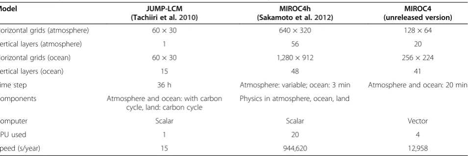
EMICs simplify the atmosphere and/or ocean by redu-cing the number of represented processes and their dimensions. Also, because EMICs generally use coarser spatial resolution in comparison to GCMs/ESMs, they run at much faster speeds than those models. For ex-ample, as in Table 2, on a scalar-type supercomputer, the EMIC Japan Uncertainty Modelling Project Loosely Coupled Model (JUMP-LCM) (Tachiiri et al. 2010; MIROC-lite component, Oka et al. 2011) ran significantly faster than the Atmosphere-Ocean GCM‘MIROC4h’, the high-resolution version of MIROC4. It is difficult to say how many times faster because it depends on the degree of parallelization and other factors. However, with the set-tings in Table 2, JUMP-LCM ran 63,000 times faster than MIROC4h, and also runs significantly faster than a GCM of a medium-resolution version of MIROC4 with the con-ditions shown in Table 2.

Based on the method of simplification, atmospheric components of EMICs may be classified into four types: 1) statistical-dynamical models, e.g., Climate-Biosphere 3α (CLIMBER-3α) (Montoya et al. 2005); 2) energy moisture

balance models (EMBM), e.g., University of Victoria (UVic) (Weaver et al. 2001); 3) quasi-geostrophic models, e.g., Loch–Vecode-Ecbilt-Clio-agism Model (LOVECLIM) (Driesschaert 2005); and 4) a new fourth type using primitive equations, e.g., Fast Met Office/UK Universities Simulator (FAMOUS) (Smith 2012). Statistical-dynamical models are based on time-averaged equations, wherein the effects of large-scale atmospheric and oceanic transi-ent eddies are parameterized in terms of climatic means or neglected (Saltzman 1978). The EMBMs are based on the vertically integrated energy-moisture balance equa-tions, and the quasi-geostrophic models are based on a quasi-geostrophic approximation. For the ocean, some use frictional geostrophic models, but many adopt primitive equation models as ocean GCMs.

In the latest EMIC intercomparison project, EMIC AR5, designed for contributing to the IPCC Fifth Assessment Report (AR5) report, there were 15 participant EMICs (http://climate.uvic.ca/EMICAR5/). Of these, four are statistical-dynamic, seven are EMBMs, two are quasi-geostrophic, and two are based on primitive equations. Seven models have a 3D atmosphere, up from three (of eight) in the Fourth Assessment Report (AR4) of IPCC (IPCC 2007). For the ocean, eight use primitive equa-tions, four use frictional-geostrophic models, and the rest are mixed-layer or box models. The model with the finest spatial resolution, UVic 2.9 (Weaver et al. 2001), has 1.8° × 3.6° grids for both the atmosphere and ocean, comparable to GCMs (the atmosphere of UVic 2.9 is, however, 2D). All but one have some type of sea ice scheme. Thirteen have carbon cycle components, 12 mar-ine, and 10 terrestrial. Of the latter, six are dynamic vege-tation models. Four models have sediment and weathering components (Eby et al. 2013). Table 3 is a classification of these models, based on the ecosystem components.

Zonal mean surface air temperature in the present cli-mate is well represented by EMICs, at least to a degree similar to GCMs (IPCC 2007). However, it is generally difficult for EMICs to represent the spatial distribution

Table 2 Model specifications and benchmarks: EMIC versus GCMs (supercomputer at JAMSTEC)

Model JUMP-LCM

(Tachiiri et al.2010)

MIROC4h (Sakamoto et al.2012)

MIROC4 (unreleased version)

Horizontal grids (atmosphere) 60 × 30 640 × 320 128 × 64

Vertical layers (atmosphere) 1 56 20

Horizontal grids (ocean) 60 × 30 1,280 × 912 256 × 224

Vertical layers (ocean) 15 48 41

Time step 36 h Atmosphere: variable; ocean: 3 min Atmosphere and ocean: 20 min

Components Atmosphere and ocean: with carbon cycle, land: carbon cycle

Physics in atmosphere, ocean, land

Computer Scalar Scalar Vector

CPU used 1 20 4

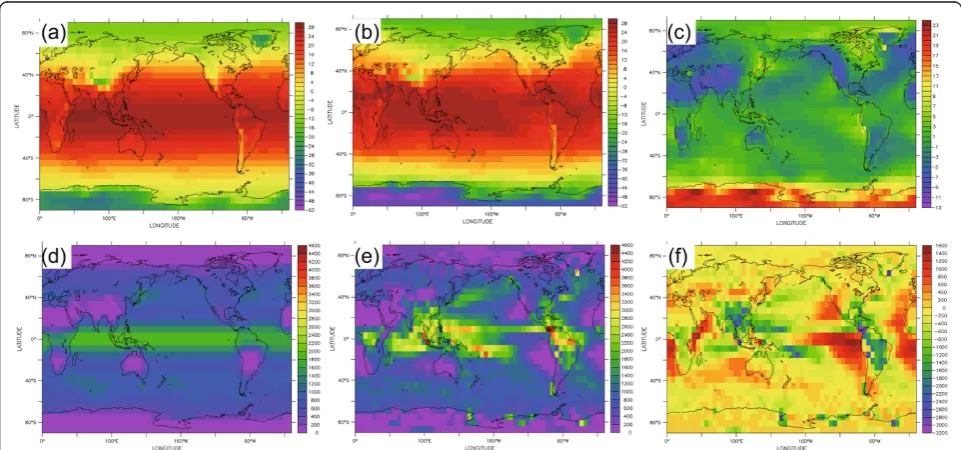
of precipitation, and so it is not easy to couple them to vegetation models. This is particularly so for EMBMs. Figure 4 shows JUMP-LCM output and a comparison with observation for atmospheric temperature and pre-cipitation. The spatial distribution of temperature is rela-tively well represented, even by the EMIC with a 2D atmosphere (Figure 4c). However, Figure 4d,e,f demon-strates the difficulty for EMICs in representing precipita-tion patterns. Figure 4d shows that the distribuprecipita-tion of

precipitation is too zonal, and there is too much precipi-tation in coastal areas and too little inland. The bias is smaller, but a non-negligible bias remains in the statistical-dynamical (e.g., Figure eight of Montoya et al. 2005) and quasi-geostrophic (e.g., Goosse et al. 2010) models. For models using primitive equations, Smith (2012) reported that their FAMOUS model had a similar but accentuated precipitation pattern relative to the mother GCM. Bias in precipitation patterns is critical with coupling to terrestrial vegetation models. To solve this problem, Tachiiri et al. (2010) used the spatial pattern of GCM output, extracted from the change in global mean surface air temperature calculated by an EMIC, to run a vegetation model.

Intercomparison of EMICs

The scope of EMICs is greatly varied. It includes large-scale ocean thermohaline circulations, biogeochemical processes, planetary atmospheres, educational use, de-bugging, and parameter tuning, with focused time scales from decades to several million years (Claussen 2005). Given this variety of model targets and output variables, the design of EMIC model intercomparison projects can be more difficult than that of GCMs/ESMs, in terms of what can or should be compared.

The first EMIC intercomparison project was EMIP-CO2(Petoukhov et al. 2005), in which eight EMICs were

involved. The modeled temperature was in relatively good agreement. However, not surprisingly, the spread of zonal precipitation was significant. In IPCC AR4, the same eight EMICs were listed (IPCC 2007), but only half overlapped

Table 3 Classification of EMICs based on ecosystem components

Ocean

No Yes

No MIROC-lite (2,3) FAMOUS (3,3) SPEEDO (3,3) MESMO 1.0 (2,3)

DCESS (box) GENIE (2,3) Yes (non-DGVM) IAP RAS CM (3,3)

IGSM2.2 (2,1) JUMP-LCMa(2,3)

Land Bern3D-LPJ (2,3)

CLIMBER-2.4 (3,2) CLIMBER-3_α(3,3) Yes (DVGM)

-LOVECLIM 1.2 (3,3) UMD 2.0 (3,2)

Uvic 2.9 (2,3) a

MIROC-lite-LCM in Eby et al. (2013). Compiled from Table one of Eby et al. (2013), based on the presence of ocean/land ecosystem components. Numbers in parentheses after model names indicate dimensions of atmosphere and of ocean. For references on each model, see Eby et al. (2013).

with EMIP-CO2. Brovkin et al. (2006) presented their

model intercomparison study results from their inter-esting experiments on the biogeophysical effects of his-torical land-cover changes during the last millennium. These results included a 0.13°C to 0.25°C global mean temperature decrease due to historical deforestation, with significant uncertainty in the zonal mean temperature and evapotranspiration.

In EMIC AR5, project protocol ranged from idealized abrupt and gradual 2xCO2and 4xCO2, historical (last

mil-lennium), to RCP experiments. Eby et al. (2013) stated that similarly to ESMs, land carbon fluxes had much more variation between models than ocean carbon. Comparison of some of their results for EMICs with those for ESMs is presented in Table 1. Equilibrium climate sensitivity and its standard deviation (SD) are similar but slightly less than those of ESMs. Climate-land carbon feedback (γL) was similar between EMICs and ESMs, but

concentration-land carbon feedback (βL) and its SD

were smaller for EMICs. In contrast, magnitudes (absolute values) of climate- and ocean concentration-carbon-cycle feedbacks (βo and γo) are larger in EMICs.

Most interestingly, the SDs of βo and γo are more than

twice those in EMICs relative to ESMs. For the last mil-lennium simulation, there was a tendency for EMICs to underestimate the decline in surface air temperature and CO2 between the Medieval Climate Anomaly and Little

Ice Age estimated from paleoclimate reconstructions (although some ESMs used different volcanic aerosol forcing).

Regarding other studies related to EMIC AR5, Weaver et al. (2012) showed that EMIC representations of the strength of the present Atlantic Meridional Overturning Circulation (AMOC) are similar to those of GCMs. In addition, Zickfeld et al. (2013) showed the result of long-term experiments for the future to the year 3000 (forced with RCPs together with their extensions to the year 2300 and then with a fixed atmospheric CO2concentration and

forcing from non-CO2greenhouse at the year 2300 levels

after that), focusing on climate change commitment and reversibility. They presented the spread of temperature rise and cumulative emission for four RCPs and indicated that the meridional overturning circulation (MOC) is weakened temporarily but recovers to near-preindustrial values in most models for RCPs 2.6 to 6.0. The MOC weakening was more persistent for RCP8.5. In compari-son to GCMs, the temperature increase projected by EMICs through the end of the twenty-first century was similar in low-concentration scenarios (RCPs 2.6 and 4.5) but significantly lower in RCP 8.5.

Existing and future studies using EMICs

Weber (2010) discussed existing studies using EMICs for the transient evolution of the climate, the AMOC

and hindcasting, assessment of uncertainties, and fore-casting. Examples of long-duration experiments include Brovkin et al. (2007), Plattner et al. (2008), Archer et al. (2009), and others dealing with the role of vegetation (Tuenter et al. 2005) and response (Claussen et al. 1999). Studies of the long-term (e.g., up to the year 3000) com-mitment of the CO2effect (Plattner et al. 2008; Zickfeld

et al. 2013) are included in this type.

Studies using large ensembles, many of which tuned pa-rameters by comparison with observations, include Knutti et al. (2002), Forest et al. (2002), Hargreaves et al. (2004), and Annan et al. (2005). Annan and Hargreaves (2010) carried out experiments of parameter perturbation, in-cluding those related to the marine carbon cycle.

For terrestrial ecosystems, Tachiiri et al. (2012) used an EMIC in a parameter perturbation experiment for a vege-tation model, identifying parameters that had significant impacts on land carbon uptake under global warming. In another type of carbon cycle-related study, Zickfeld et al. (2011) examined the nonlinearity of climate- and concentration-carbon cycle feedback using UVic-ESM.

Related to the carbon cycle, a relatively new type of study using EMICs addresses climate stabilization, through emission reduction (Matthews and Caldeira 2008) or geoengineering (Brovkin et al. 2009). A policy-oriented study using an EMIC and IAM was presented by Van Vuuren et al. (2008), and Webster et al. (2012) discussed climate policy targets under uncertainty using an EMIC.

An important advantage of EMICs (at least those with an EMBM-type atmosphere) is that we can easily vary climate sensitivity (Plattner et al. 2001; Tachiiri et al. 2010). Through this, we can assess the effect of uncer-tainty in climate sensitivity on ecosystems and then on the amount of emission following given concentration pathways. An example is Tachiiri et al. (2013) who pre-sented the potential of constraining physical properties of Earth systems using carbon-cycle related observations (in their case, carbon emission). However, they stated that this should be done very carefully because the posterior probability distribution function of physical pa-rameters is sensitive to the characteristics of ecosystem components.

EMIC importance is declining. On the contrary, this is the route toward a meaningful‘model hierarchy’, where EMICs are effectively used for sensitivity tests and tuning parameters with large ensembles to improve the perform-ance of the mother GCM/ESM. Due to this interactive connection between, or hybrid use of, EMICs and GCMs/ ESMs, complementary relationships between these models are expected in the future.

Climate geoengineering

Although understanding of anthropogenic climate change is steadily deepening, the political response has been slow and inadequate, which has led to a call for more drastic actions such as climate geoengineering. The newly re-leased AR5 of IPCC (2013) has reviewed these schemes in a comprehensive manner for the first time in its history. In this section, we restrict the discussion to scientific aspects of geoengineering, although there are considerable controversies regarding its role in society. Interested readers are referred to the Royal Society (2009) and IPCC (2012) and references therein.

There are useful references on the science of geoengi-neering, such as Caldeira et al. (2013) and chapters 6 and 7 of IPCC Working Group 1 of AR5. In the following, we focus on the modeling of geoengineering techniques.

Definitions

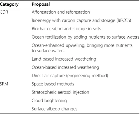
According to the IPCC, geoengineering is defined as ‘a broad set of methods and technologies that aim to delib-erately alter the climate system in order to alleviate the impacts of climate change’(see the IPCC glossary). This is different from other responses to climate change such as mitigation (reductions of greenhouse gas emissions) or adaptation (moderating the damage by changing soci-etal practice and behavior). Geoengineering is often di-vided into solar radiation management (SRM) and carbon dioxide removal (CDR). Table 4 lists categories of pro-posed schemes, based on the classification of the IPCC (2013).

SRM is intended to reflect some incoming solar radi-ation back to space, e.g., by spraying scattering aerosol particles in the stratosphere (Rasch et al. 2008), bright-ening clouds (Latham 1990), using a mirror system in space (Angel 2006), or increasing surface albedo (Lenton and Vaughan 2009). There are related schemes, such as a reduction in cloud forcing of cirrus clouds (Mitchell and Finnegan 2009).

CDR (or negative emissions technology, NET) refers to a class of techniques that reduce atmospheric CO2

concentration either by increasing natural carbon sinks or directly removing CO2via industrial engineering. The

proposed schemes include bioenergy with carbon cap-ture and storage (BECCS), direct air capcap-ture through chemical engineering, storing biochar in soils, and the

acceleration of chemical weathering, which in nature ab-sorbs CO2on a geologic time scale. Because the definition

of mitigation covers the enhancement of natural sinks (e.g., afforestation and reforestation), there is some overlap between geoengineering and conventional mitigation. In fact, the simulation of RCP2.6 by an IAM, IMAGE, as-sumes widespread use of BECCS. Therefore, CDR may not necessarily represent an additional CO2reduction

op-portunity. Theoretically, one can achieve removal of non-CO2greenhouse gases, though literature on this is scarce.

Among the many proposed SRM schemes, the two most discussed are stratospheric aerosol injection and cloud brightening. The current understanding of the former is primarily based on climate response to volcanic forcing, and the latter on cloud processes and physics. For the CDR schemes, ocean iron fertilization has historically received great attention. The three schemes in this para-graph are relevant to ESS and modeling.

Characteristics

Although various techniques are grouped under the ru-bric of geoengineering, they have vastly different charac-teristics with respect to effectiveness, environmental risks, and other aspects. As Keith et al. (2010) summa-rizes, SRM has the following features. Its implementa-tion is usually of low cost and, once initiated, can cool the climate rapidly. However, its ability to counteract climate change is imperfect and cannot offset all its impacts. Further, the science is rudimentary and all aspects of SRM are uncertain.

Take the example of stratospheric aerosol injection. This technique is believed to be capable of counteracting a doubling of CO2rapidly and cheaply. However, it has

side effects, including ozone destruction, slowdown of the global hydrologic cycle, and reduction of electricity

Table 4 Categories of geoengineering proposals, based on IPCC (2013)

Category Proposal

CDR Afforestation and reforestation

Bioenergy with carbon capture and storage (BECCS) Biochar creation and storage in soils

Ocean fertilization by adding nutrients to surface waters Ocean-enhanced upwelling, bringing more nutrients to surface waters

Land-based increased weathering Ocean-based increased weathering Direct air capture (engineering method) SRM Space-based methods

Stratospheric aerosol injection Cloud brightening

generation by concentrating solar power. If the injection were ever halted suddenly, it could result in a sudden rise in the global mean surface temperature by unmask-ing radiative forcunmask-ing of greenhouse gases. This technique also fails to address ocean acidification.

The characteristics of CDR can be understood by com-parison with SRM. CDR is more expensive, slower to affect the carbon cycle, but more reliable because it in-fluences the real culprit of climate change. However, some schemes, especially those that intervene in the ecological system, are certain to have significant side ef-fects. Cost estimates tend to be comparable to or higher than conventional mitigation.

For example, the direct air capture of CO2is

consid-ered to have great potential for atmospheric CO2

reduc-tion. Although technology exists, it is not clear whether it can be operated on an industrial scale because the cost estimate is very uncertain, but it is at least as expensive as conventional mitigation.

Modeling of CDR

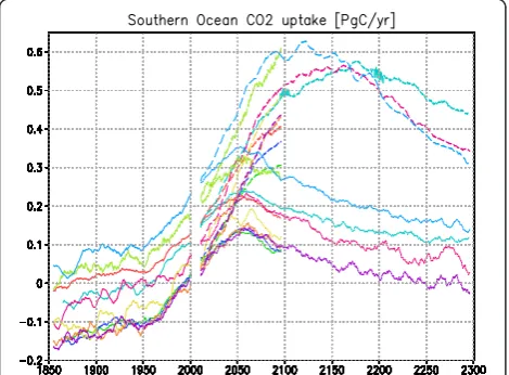
Martin (1990) put forth a hypothesis that iron is the lim-iting factor in high-nutrient, low-chlorophyll (HNLC) re-gions such as the Southern Ocean, the equatorial Pacific, and the North Pacific. Since then, about a dozen small-scale (O(100 km2)) in situexperiments have been con-ducted (Strong et al. 2009). Because these intervention experiments have vindicated the iron hypothesis, there was growing interest in iron fertilization of oceans for CO2 reduction (see also ‘Atmospheric deposition of

bioavailable iron in marine ecosystems’section).

Several modeling studies have evaluated ocean fertiliza-tion with varying degrees of sophisticafertiliza-tion. Earlier studies, which used biogeochemical cycle models without the explicit iron cycle, implicitly modeled the effect of iron fertilization, e.g., by depleting near-surface phosphate (Sarmiento and Orr 1991). These studies tended to report optimistic potentials for atmospheric CO2drawdown, and

some reported approximately 100 ppm of CO2drawdown

(Joos et al. 1991; Cao and Caldeira 2010b). As the models improved, however, estimates of the potential were revised downward in most studies. For example, Aumont and Bopp (2006) ran a biogeochemical cycle model with the iron cycle, obtaining a drawdown of 33 ppm (Aumont and Bopp 2006). Similarly, Sarmiento et al. (2010) reported 42 ppm. One reason for such differences is that there are non-iron limiting factors such as silicate and light, and carbon export to the deep ocean can only occur during the growing season (Aumont and Bopp 2006).

In addressing the amount of atmospheric removal, we must consider the ‘rebound effect’. When human activ-ities cause CO2 emissions into the atmosphere, only

about half remains there, with the rest absorbed by

terrestrial and oceanic sinks. When human activity removes CO2from the atmosphere, the opposite occurs.

To reduce the CO2concentration by 1 ppm, for example,

one needs to take up an amount of CO2 equivalent to

approximately 2 ppm (assuming that the airborne fraction is approximately 0.5). This has been termed the rebound effect, and one must be careful about the efficacy of CDR (Cao and Caldeira 2010a).

The ocean fertilization potentials reported above ac-count for the rebound effect from the oceans but exclude the effect from land, thereby overestimating the potential.

Another use of ESMs is to calculate required emission reductions compatible with a certain target RCP. Cumu-lative emissions compatible with RCP2.6 are estimated at 272 ± 101 PgC for the period 2012 to 2100 (chapter 6 of IPCC Working Group 1 of AR5, IPCC 2013). Some results suggest that sustained negative emissions, such as those from BECCS, are required.

Modeling of SRM

Process studies and engineering analyses have indicated that it would be feasible to conduct SRM for canceling a CO2doubling and that the current cost of

implementa-tion is inexpensive, at least for stratospheric aerosol injection. Significant uncertainty remains, however, as to its efficacy of counteracting climate change and its side effects. Modeling can therefore make an important con-tribution to the evaluation of geoengineering schemes.

The situation of SRM modeling was rudimentary until the advent of the Geoengineering Model Intercompari-son Project (GeoMIP), which is related to CMIP5 activ-ities. One of the motivations for this project was the impact of geoengineering on the Asian summer mon-soon (Kravitz et al. 2011). Some models implied a sub-stantial decrease in monsoon precipitation, while others suggested the opposite. However, the number of models in the exercise was small and scenario specifications varied, complicating the interpretation. Obviously, a more systematic approach to modeling was needed.

The initial GeoMIP included the following four experiments:

G1: Cancel the warming from instantaneous CO2 quadrupling with a simultaneous decrease of the solar constant

G2: Counteract warming from CO2increase at 1% per year by steadily reducing the solar constant G3: Starting in 2020, offset RCP4.5 forcings by

gradually increasing the amount of SO2or sulfate injected either at the equator or globally

This set of experiments had variable scenario com-plexities to attract many modeling groups, with two ex-periments focusing on the solar constant and the other two on the injection of sulfates. In CMIP5, most models used an externally specified optical depth to represent volcanic cooling, but models in GeoMIP represent a variety of approaches, from the CMIP5-type approach to directly simulating stratospheric chemistry and aerosols.

In the following, we summarize the 12-model G1 experiment by Kravitz et al. (2013a), which confirmed basic results of previous studies. Twelve fully coupled AOGCMs were included, 11 of which came with a land ecosystem model. The required solar constant reduction was model-dependent, between 3.5% and 5.0%.

The G1 results show that a reduction of solar insolation can largely offset the temperature changes but leave the polar region warmer (inter-model average 0.8 K) and the tropics colder (inter-model average−0.3 K) than preindus-trial levels (Figure 5). This is because a reduction of solar insolation by the same fraction led to a large-magnitude reduction in equatorial regions. Similarly, net precipitation (precipitation minus evaporation) induced by quadrupling CO2could be mostly offset by the reduction of solar

in-solation, although there was less precipitation in some

tropical regions. The tropical precipitation is explained by changes in moist static stability. Quadrupling CO2

increases net primary productivity because of CO2

ferti-lization effects. In the G1 results, net primary product-ivity increases a little more, because geoengineering creates an artificial environment in which the CO2level

is elevated and climate change is reduced.

GeoMIP has investigated other topics related to cli-mate geoengineering, such as changes in the hydrologic cycle, extreme events, stratospheric ozone loss, and im-pacts on agriculture and the cryosphere. The results have been published in a special issue of the Journal of

Geophysical Research (Kravitz et al. 2013b). GeoMIP

research teams are discussing the next round, which includes experiments on cloud brightening.

Remaining uncertainties

Although initial evaluations of CDR and SRM tech-niques are useful, there remain substantial uncertainties in various types of geoengineering method. GeoMIP made great progress in stratospheric aerosol injection and had a plan for cloud brightening as well. Neverthe-less, there have been no model intercomparison projects for CDR. If governments and society were to consider

Figure 5Impacts of solar radiation management evaluated by ESMs.Zonal-mean anomalies of surface air temperature in kelvin (land and ocean; 12 models), precipitation minus evaporation in millimeters per day (land average; 12 models), and terrestrial net primary productivity in kg C per m2_{per year (land average; 8 models) for all available models. All values are averages over years 11 to 50 of the simulations. Horizontal axis}