Just-in-time preemptive single machine problem with costs of earliness/tardiness, interruption and work-in-process Pages 321-336 Download PDF

(1)

* Corresponding author Cell phone: +98-9363767625

doi: 10.5267/j.ijiec.2011.11.004

International Journal of Industrial Engineering Computations 3 (2012) 321–336

Contents lists available at GrowingScience

International Journal of Industrial Engineering Computations

homepage: www.GrowingScience.com/ijiec

Just-in-time preemptive single machine problem with costs of earliness/tardiness, interruption and work-in-process

Mohammad Kazemia, Elnaz Nikoofaridb, Amin Aalaeic* and Reza Kiad

a

Department of Industrial Engineering, Birjand University of Technology, Birjand, Iran

b

Department of Industrial Engineering, Mazandaran University of Science & Technology, Babol, Iran

c

Department of Industrial Engineering & Management Systems, Amirkabir University of Technology, Hafez Ave, Tehran, Iran

d

Department of Industrial Engineering, Firoozkooh Branch, Islamic Azad University

A R T I C L E I N F O A B S T R A C T

Article history:

Received 20 October 2011 Received in revised form November, 2, 2011

Accepted November, 18 2011 Available online

28 November 2011

This paper considers preemption and idle time are allowed in a single machine scheduling problem with just-in-time (JIT) approach. It incorporates Earliness/Tardiness (E/T) penalties, interruption penalties and holding cost of jobs which are waiting to be processed as work-in-process (WIP). Generally in non-preemptive problems, E/T penalties are a function of the completion time of the jobs. Then, we introduce a non-linear preemptive scheduling model where the earliness penalty depends on the starting time of a job. The model is liberalized by an elaborately–designed procedure to reach the optimum solution. To validate and verify the performance of proposed model, computational results are presented by solving a number of numerical examples.

Just-in-time Preemption Earliness/Tardiness Interruption Penalties Work-In-Process Single Machine Scheduling

1. Introduction

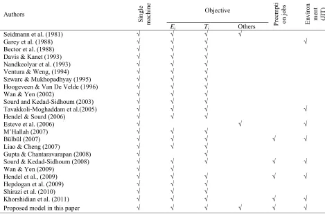
In the single machine scheduling problem with E/T, a set of jobs, each with an associated due date, has to be scheduled on a single machine. Each job has a penalty per unit time associated with completing before its due date, and a penalty per unit time associated with completing after its due date. There are many extensive efforts in the recent years to minimize the weighted number of early and tardy jobs in single machine scheduling problem (Seidmann et al. 1981; Bector et al. 1988; Davis & Kanet, 1993; Nandkeolyar et al. 1993; Ventura & Weng, 1994; Szwarc & Mukhopadhyay, 1995; Hoogeveen & Van De Velde, 1996; Wan & Yen, 2002; Luo et al. 2006; Hendel & Sourd, 2006; Liao & Cheng, 2007; Sourd & Kedad-Sidhoum, 2003).

(2)

Gupta and Chantaravarapan (2008) presented a mixed-integer linear programming model for single machine scheduling problem considering independent family (group) setup times where jobs in each family are processed together. A sequence-independent setup time is required to process a job from a different family.

Wan and Yen (2009) considered a single machine scheduling problem to minimize the total weighted earliness subject to minimum number of tardy jobs. They developed a heuristic and a branch and bound algorithm and compared these two algorithms for problems in different sizes. Hepdogan et al. (2009) Investigated a meta-heuristic solution approach for the early/tardy single machine scheduling problem with common due date and sequence-dependent setup times.

The objective of this problem is to minimize the total amount of earliness and tardiness of jobs, which are assigned to a single machine. Shirazi et al. (2010) proposed a new approach called Tabu-Geno-Simulated Annealing (TGSA) by hybridization of three well-known metaheuristics for solving single machine scheduling problem for a common due date with arbitrary E/T penalties. The objective is to determine the common due date and processing sequence of new jobs together with the re-sequencing of old jobs to minimize the sum of total E/T, completion time, and due date related penalties.

2. Literature review

Just-in-time (JIT) scheduling problems establish a well-studied class of multi-criteria scheduling problems. Indeed, these problems with earliness penalties are very useful to represent practical problems, in which either perishable goods should be delivered or storage costs should be regarded. Tardiness, Ti, and earliness, Ei, are computed by:

• Ti= max (0, Ci - di),

• Ei = max (0, di - Ci),

where Ci and di denote the completion time and due date of job i, respectively. Clearly, a task cannot

simultaneously have a positive tardiness and a positive earliness; a task is either tardy or early. Moreover, earliness and tardiness are often similar in terms of costs induced by a delivery that is not on time. Therefore, these two criteria are often aggregated into a single criterion fi(Ci)= aiEi + biTi,

which is called the weighted deviation of the task with respect to its due date. Interestingly, this deviation function can be generalized to express more complex combinations of contradicting criteria and soft or hard constraints on the due date obligated by a customer. Garey et al. (1988) proposed a direct algorithm based on the blocks of adjacent jobs with computational complexity O(n log n), valid

for the JIT problem with symmetric earliness and tardiness penalties.

Tavakkoli-Moghaddam et al. (2005) studied a single machine scheduling problem to minimize the sum of maximum earliness and tardiness by considering idle insertion. The proposed model, which could be adapted by production systems such as JIT presented the optimal solutions. Additionally, the authors developed a number of effective lemmas regarding idle insertion. For this type of scheduling models, Tavakkoli-Moghaddam et al. (2006) introduced a branch-and-bound algorithm to solve the problems, where a suitable lower and upper bound were represented. To show the effectiveness of the proposed algorithm, they generated and solved different sizes of the model. Esteve et al. (2006) studied the problem of scheduling JIT with a set of jobs on a single machine to minimize the mean weighted deviation from distinct due dates. Recovering Beam Search algorithm was proposed by the authors to show the efficiency of the solution approach.

(3)

tardiness to capture the JIT philosophy, where the earliness costs depend on the start times of the jobs and tardiness costs depend on completion times. They applied an efficient representation of dominant schedules and introduced a polynomial algorithm to compute the best schedule for a given representation. By using local search algorithm and a branch-and-bound procedure, the authors showed there is a very small gap between their results and optimum solutions. Runge and Sourd (2009) addressed a new model for the single machine E/T scheduling problem where preemption is allowed. In this model, presented interruption costs are based on the WIP of the job. The WIP costs are based on the differences among the start and completion times of the jobs. This model presented two main advantages over an existing model HS presented by Hendel and Sourd (2005).

Primary, HS does not penalize interruption in all cases. And the next advantage is that liberty among the E/T and the WIP costs allows them to design a new timing algorithm with a better time complexity. Also they discussed for several dominance rules and the particular case of the scheduling problem around a common due date. Furthermore, presented the lower bound for the timing algorithm and explained that a local search algorithm based on their new timing algorithm is sooner than a local search algorithm, which uses the timing algorithm presented by Hendel and Sourd (2005). Khorshidian et al. (2011) presented a new mathematical model in the expansion of the classical single machine E/T scheduling problem where preemption is allowed and idle time is also considered. The proposed model finds the sequence configuration with the aim of minimizing the scheduling costs. An efficient algorithm based on genetic algorithm (GA) was planned to solve the mathematical model. Schematic representation of literature review for problem definition is illustrated in Table 1.

Table 1

Scheduling attributes used in the present research and in a sample of published articles

Authors

Sin

gle

mach

ine _Objective

Pr

eempti _{on jo}

bs

Envi

ro

n

me

nt

(JIT)

Ei Ti Others

Seidmann et al. (1981) √ √ √ √

Garey et al. (1988) √ √ √ √

Bector et al. (1988) √ √ √

Davis & Kanet (1993) √ √ √

Nandkeolyar et al. (1993) √ √ √

Ventura & Weng, (1994) √ √ √

Szwarc & Mukhopadhyay (1995) √ √ √ Hoogeveen & Van De Velde (1996) √ √ √

Wan & Yen (2002) √ √ √

Sourd and Kedad-Sidhoum (2003) √ √ √

Tavakkoli-Moghaddam et al.(2005) √ √ √ √

Hendel & Sourd (2006) √ √ √

Esteve et al. (2006) √ √ √

M’Hallah (2007) √ √ √

Bülbül (2007) √ √ √ √ √

Liao & Cheng (2007) √ √ √

Gupta & Chantaravarapan (2008) √ √

Sourd & Kedad-Sidhoum (2008) √ √ √ √ √

Wan & Yen (2009) √ √

Hendel et al., (2009) √ √ √ √ √

Hepdogan et al. (2009) √ √ √

Shirazi et al. (2010) √ √ √

Khorshidian et al. (2011) √ √ √ √ √

(4)

Runge and Sourd (2009) calculated the total interruption and WIP penalties by the “idle” time (for job Ji) is equal to Ci −Si −pi. However, in our model, we calculate the number of interruption and

work-in-process of each jab, separately. In addition, in our model, WIP penalties are commensurate with percentage of a process improvement for each job, in other word, if a job is interrupted, the time this job spends on the machine is extended and WIP increases.

The remainder of this paper is organized as follows. In Section 3, a new mathematical model is presented for a single machine scheduling problem in JIT system where preemption and idle times are allowed, with E/T penalties, interruption penalties and holding cost of jobs which are waiting to be processed as work in process (WIP). The linearization procedure and the liberalized model are presented in Section 4. Section 5 shows the numerical examples to validate and verify the performance of proposed model. Finally, conclusion is given in Section 6.

3. Problem formulation

3.1. Problem description

In this section, a nonlinear programming mathematical model of a single machine scheduling problem with preemptive jobs in JIT environment to minimize the total tardiness-earliness penalties, interruption penalties and holding cost of jobs which are known as work- in-process is proposed. Since this model permits preemption, we have to add a term to the objective function, which penalizes the interruption of jobs. Certainly, if a job is interrupted, the time this job spends on the machine is extended and work-in-process increases. We assume that the processing times, starting times and due dates are integer numbers. The problem is formulated according to the following assumptions.

1. The processing time for each job is known and deterministic. 2. Only one job can be processed on the machine simultaneously. 3. A job can be processed by the machine if it is idle.

4. The preemption of jobs is allowed.

5. Completing a job before its due date is not allowed. 6. Number of jobs to be processed is constant.

7. Work-in-process is allowed and its associated cost is considered.

8. More processed job will incur more cost of work-in-process if it is interrupted. 9. The interrupt cost of each job is considered.

10.Machine setup time is negligible.

11.The machine will never breakdown and be available throughout the scheduling period.

Consider a non-preemptive single machine scheduling problem with scheduling problem with just-in-time (JIT) approach. Associated with each job i , i = 1, . . . , N, are several parameters: Pi , the

processing time for job i ; Dic , the due date for job i ; βi, the tardiness cost per unit time if job i

completes processing after Dic ; and earliness costs as Ei = max(0, Dis - Si ) where this penalty

depends on the starting time of a job; Si where is the start time of job i ; and Dis= Dic- Pi +1 is the

ideal start time for job i (that is the target start time); andα_i, the earliness cost per unit time if job i

starts processing before Dis . We assume that the processing times, start times and due dates are

integers.

3.2. Notations

3.2.1. Subscripts

(5)

J Number of position i Index for job (i=1,2,…N) j Index for position (j=1, 2,…J)

3.2.2. Input parameters

Pi Processing time of job i,

Dic The ideal completion time (or due date) of job i,

i

α

The unitary earliness penalty of job i if itstarts processing before Dis, i

β

The unitary tardiness penalty of job i if itcompletes processing after Dic,

i

γ

Unit cost of work-in-process holding of job i,

i

η

The unitary interruption penalty of job i,

A An arbitrary big positive number.

3.2.3. Decision variables

Ci Completion time of job i,

Dis Ideal starting time for job i which is computed as Dis= Dic - Pi +1,

Xij 1 if job i is processed in position j, and 0 otherwise,

Ei Earliness of job i,

Ti Tardiness of job i,

Si Starting time of job i.

3.3. Mathematical model

min Z =

1

( )

N

i i i i

i E T α β = +

∑

(1.1) 1 1 1 1 1 1 . 2 2 N J

i ij ij iJ i

i j

X X X X

η

− ₊ = = ⎡⎛ ⎞ ⎤ + _⎢_⎜ − _⎟+ + − _⎥ ⎢⎝ ⎠ ⎥ ⎣ ⎦

∑

(1.2)

1 1

.( ).

N J

ij i i

i j

X C j γ

= =

+

∑∑

− _(1.3)

subject to 1 J ij i j X P = =

∑

∀i; (2)

1 1 N ij i X = ≤

∑

∀i; (3)

c

i i i

T ≥C −D ∀i; (4)

s

i i i

E ≥D −S ∀i; (5)

{ }

0,1

ij

X ∈ ∀i j, ; (6)

, 0 i i

T E ≥ ∀i; (7)

max( . )

i _j ij

C = X j _∀_i_; ₍₈₎

min (1 )

i ij

j

S = ⎡_⎣j+A −X ⎤_⎦ ∀i; (9)

(6)

C1

the third component takes into account the holding cost of all jobs which are waiting to be processed as works in process. Equality (2) guarantees that the number of positions in which job i is processed

is equal to the processing time of job i. Inequality (3) necessitates that in each position only one job is

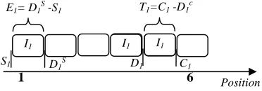
processed. The tardiness and earliness of each job are calculated by Constraints (4) and (5). Constraints (6) and (7) provide the logical binary and non-negativity integer necessities for the decision variables. Eq. (8) and Eq. (9) present the completion time and starting time of each job, respectively. In the following, the components of objective Fig 1 shows an example to illustrate the calculation way of earliness and tardiness in the first component of objective function and related constraints (4) and (5). As we can see, the completion time of job 1 (C1) happens after its due date

(D1c). As a result, tardiness of job 1 happens and its value is equal to T1 = C1 - D1c. Also, the starting

time of job 1 (S1) happens before its ideal starting time (D1s). Therefore, earliness of job 1 happens

and its value is equal to E1 = D1s - S1. The cost resulted from E/T is obtained by product unitary E/T

penalty and the related E/T quantities.

1 6

Fig. 1. Earliness and Tardiness cost

In the second component of objective function, the interruption cost is calculated by product the number of interruptions on the machine and the unitary interruption penalty. By considering that variable Xij is binary, one of the following situations will happen in term

1

1 1

J

ij ij

j

X X

−

+ =

−

∑

of the

second component of objective function:

1. If X_ij =1 and X_ij₊₁=1, the absolute term returns 0 as the result which implies job i in

positions j and j+1 is processed on machine without any interruption.

2. If X_ij =1 andX_ij₊₁=0, the absolute term returns 1 as the result which implies job i is

processed in position j but not in position j+1. Therefore, an interruption happens between

positions j and j+1 for job i.

3. If X_ij =0and X_ij₊₁=1, the absolute term returns 1 as the result which implies job i is not

processed in position j but in position j+1. Therefore, an interruption happens between

4. If X_ij =0 and X_ij₊₁=0, the absolute term returns 0 as the result which implies job i in

positions j and j+1 is not processed on machine. Therefore, there is no interruption between

If the starting position in which job i starts to be processed is any position except the beginning

position 1, term 1 ₁

1 J

ij ij

j

X X

−

+ =

−

∑

takes into account an interruption while it doesn’t happen in reality.

Similarly, if the final position in which job i completes its process is any position except the ending

position J, term

1

1 1

J

ij ij

j

X X

−

+ =

−

∑

takes into account an interruption while it doesn’t happen in reality.

To overcome this fault in calculating the number of interruptions, 2 units are subtracted from

1

1 1

J

ij ij

j

X X

−

+ =

−

∑

. Since for a job variables X_i₁ or X_iJ may be equal to 1 that means the job is

I1 I1

Position I1

D1

T1=C1 -D1c

E1= D1S -S1

(7)

I1

I1 I1

Positions

C1

Positions I1

I1 I1

processed on the beginning or ending position, then it shouldn’t to subtract 2 units from term

1 1 1 J ij ij j X X − + = −

∑

and Xi1 or XiJ should be added to nullify the effect of that subtracting. Term

1

1 1

2

N J

ij ij iJ i

i j

X X X X

− + = = ⎡⎛ ⎞ ⎤ − + + − ⎢⎜ ⎟ ⎥ ⎢⎝ ⎠ ⎥ ⎣ ⎦

∑ ∑

takes into account the number of interruptions twice its real

value, therefore to reach the true number of interruptions the final value of that term should be divided to 2.

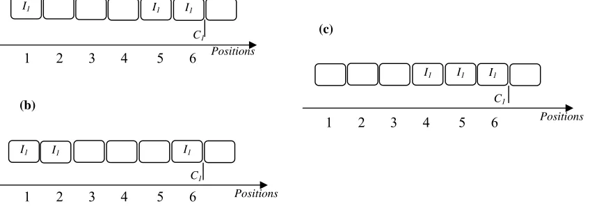
To validate the presented formula for calculating the number of interruptions, two examples for job 1 with processing time 3 are presented. In the first example two interruptions and in the second example one interruption happens.

.

1 6 1 6

Fig. 2. Two examples to calculate the number of interruptions

As we can see, in the first example, one interruption happens between positions 2 and 3 and the other happens between positions 5 and 6. Also, in the second example only one interruption happens between positions 3 and 4. The number of interruptions for the first example based on the presented formula is as below:

1 6 1

1 1

1

.[((|1 0 |) (| 0 1|) (|1 0 |) (| 0 0 |) (| 0 1|)) 1

. 2

2 ij ij i i 2 1 1 2] 2

i j

X X X X

− + = = ⎡⎛ ⎞ ⎤ − + + − ⎢⎜ ⎟ ⎥ ⎢⎝ ⎠ ⎥⎦= − + − + − + − + − + + − = ⎣

∑ ∑

and for the second example is 1.[((| 0 1|) (|1 0 |) (| 0 1|) (|1 1|) (|1 0 |)) 0 0 2] 1.

2

= − + − + − + − + − + + − =

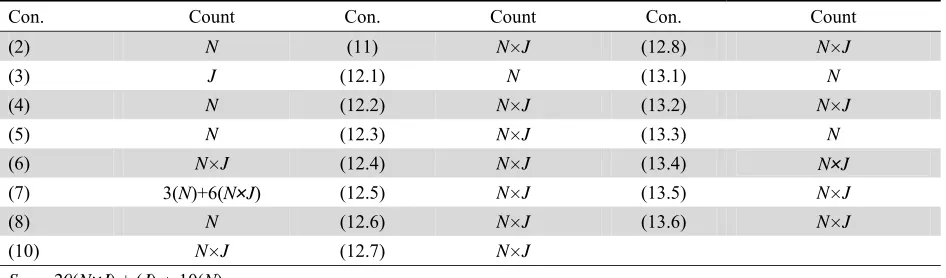
It is proved that the presented formula calculates the number of interruptions exactly. In the third component of the objective function, the holding cost of all jobs which are waiting to be processed as works in process is computed. This component tries to complete a job after it starts to be processed as soon as possible. Also, it aims to interrupt a job in the preliminary positions of its process provided that the job is interrupted because of assumption 13. Fig 3 shows the effect of the interruption times of a job on the work-in-process holding cost in the third component of the objective function. In all three cases of this example, job 1 with process time 3 completes its process in position 6.

1 2 3 4 5 6

Fig. 3. The effect of the work in process cost

(a) (b)

I1

Positions Positions I1 I1 (b) (c) I1 C1

I1 I1

C1

Positions

(8)

The work-in-process holding costs for all three cases are calculated as follows. That is for case (a):

1 7

1 1

[1.(6 1) 0.(6 2) 0.(6 3) 0.(6 4) 1.(6 5) 1.(6 6)].

.( ). 6

ij i i

i j

X C j γ γ γ

= =

− + − + − + − + − + −

= =

−

∑∑

That is for case (b):

1 1

[1.(6 1) 1.(6 2) 0.(6 3) 0.(6 4) 0.(6 5) 1.(6 6)].− + − +

γ

9

γ

= − + − + − + − =

That is for case (c):

1 1

[0.(6 1) 0.(6 2) 0.(6 3) 1.(6 4) 1.(6 5) 1.(6 6)].− + − +

γ

3

γ

= − + − + − + − =

The flow time for cases (a) and (b) is 6 and for case (c) is 3. Therefore, in case (c) a less holding cost

is incurred in compare to cases (a) and (b) which is equal to3

γ

₁. The second time unit of process for

case (a) is done in position 5 and for case (b) is done in position 2. Then, the amount of

work-in-process in case (b) is more than it in case (a) and consequently it incurs more holding cost in compare

to case (a) based on assumption 13.

4. Linearization of the proposed model

In this section, we present the linearization procedure and the liberalized model.

4.1. Linearizationprocedure

The linearization procedure that we propose here consists of four steps that are given by the four propositions stated below. Terms (1.2), (1.3), (8) and (9) are non-linear, therefore, these four terms will be liberalized using the following auxiliary variables XPij, XMij, Mij, Qij, Rij, Fij and Bij. Each

proposition for linearization is followed by a proof that illustrates the meaning of each auxiliary (linearization) variable and additional constraints.

Proposition1. The non-linear term of the objective function (1.2) can be liberalized by the following transformationX_ij −X_ij₊₁ =X P_ij +X M_ij , under the following set of constraints:

1 , ;

ij ij ij ij

X −X ₊ = XP −XM ∀i j (10)

The proof of this proposition is given in Appendix A.

Proposition2. The non-linear work-in-process holding cost terms in the objective function (1.3) can be liberalized withX_ij.(C_i − j)=M_ij, under the following set of constraints:

( ) (1 ) , ;

ij i ij

M ≥ C − −j A −X ∀i j (11)

The proof of this proposition is given in Appendix B.

Proposition3. The non-linear constraint (8) can be liberalized by the following transformation

max( ij. ) iJ

j X j =Q , under the following sets of constraints:

1 1 ;

i i

Q = X ∀i (12.1)

1.(1 ) ( . ) , ;

ij ij ij ij

Q =Q ₋ −X + j X ∀i j (12.2)

The proof of this proposition is given in Appendix C.

Proposition4. The non-linear constraint (9) can be liberalized by adding the following set of

(9)

1 1 ;

i i

B = X ∀i (13.1)

1 (1 1). , ;

ij ij ij ij

B =B ₋ + −B ₋ X ∀i j (13.2)

1

1 ;

J

i ij

j

S J B i

=

= −

∑

+ ∀ (13.3)

The proof of this proposition is given in Appendix D.

4.2. The liberalized model

We now present the linear mathematical model as follows:

minz =(1.1)

1 1 1 1 1 . 2 2 N J

i ij ij iJ i

i j

X P X M X X

η

− = = ⎡⎛ ⎞ ⎤ + ⎢⎜ + ⎟+ + − ⎥ ⎢⎝ ⎠ ⎥ ⎣ ⎦

∑

(1.2')

1 1 . N J ij i i j M γ = =

+

∑∑

(1.3')

Subject to:

(2), (3), (4), (5)

{ }

, , 0,1 ij ij ij

X P XM X ∈ ∀i j, ; (6)

, , , , , , , , 0

ij ij ij ij ij ij i i i

G B F Q R M C T E ≥ ∀i j, ; (7)

i iJ

C =Q ∀i; (8)

1

ij ij ij ij

X −X ₊ =X P −X M ∀i j, ; (10)

( ) (1 )

ij i ij

M ≥ C − j −A −X ∀i j, ; (11)

1 1

i i

Q =X ∀i; (12.1)

1

ij ij ij ij

Q =Q ₋ −R +F ∀i j, ; (12.2)

1 (1 )

ij ij ij

R ≤Q ₋ +A −X ∀i j, ; (12.3)

1 (1 )

ij ij ij

R ≥Q ₋ −A −X ∀i j, ; (12.4)

.

ij ij

R ≤A X ∀i j, ; (12.5)

(1 )

ij ij

F ≤ +j A −X ∀i j, ; (12.6)

(1 )

ij ij

F ≥ −j A −X ∀i j, ; (12.7)

.

ij ij

F ≤A X ∀i j, ; (12.8)

1 1

i i

B =X ∀i; (13.1)

1

ij ij ij ij

B =B ₋ +X −G ∀i j, ; (13.2)

1

J

i ij

j

S J B

=

= −

∑

+ ∀i; (13.3)

1 (1 )

ij ij ij

G ≤B ₋ +A −X ∀i j, ; _(13.4)

1 (1 )

ij ij ij

(10)

.

ij ij

G ≤A X ∀i j, ; (13.6)

The number of variables and constraints in the liberalized model are presented parametrically in Tables 1 and 2 respectively, based on the variable indices.

Table1

The number of variables in the liberalized model

Count Variable Count Variable Count Variable N×J Rij N×J Mij N×J Xij N×J XPij N×J Fij N Ti N×J XMij N×J Bij N Ei N×J Gij N×J Qij

Sum= 2 (N) +9 (N×J)

Table 2

The number of constraints in the liberalized model

Count Con. Count Con. Count Con. N×J (12.8) N×J (11) N (2) N (13.1) N (12.1) J (3) N×J (13.2) N×J (12.2) N (4) N (13.3) N×J (12.3) N (5)

N×J

(13.4) N×J (12.4) N×J (6) N×J (13.5) N×J (12.5) 3(N)+6(N×J)

(7) N×J (13.6) N×J (12.6) N (8) N×J (12.7) N×J (10)

Sum=20(N×J) + (J) + 10(N)

5. Numerical examples

To validate the proposed model, a numerical example in a small size with randomly generated data is solved by a branch-and-bound (B&B) method under the Lingo 11.0 software on an Intel® CoreTM2.4 GHz Personal Computer with 4 GB RAM. Table 3 presents the information related to each job in this example and contains processing time, due date, the penalty of earliness, tardiness, and interruption as well work-in-process holding cost.

Table 3 Job information

Job

number Processing Time Due date Ideal Start Time Earliness Penalty Tardiness Penalty Interruption penalty Work-in-process holding cost

1 4 9 6 80$ 60$ 5$ 1$

2 6 12 7 60$ 40$ 8$ 2$

3 4 12 9 80$ 90$ 6$ 5$

4 5 17 13 70$ 80$ 3$ 2$

5 5 29 25 60$ 50$ 2$ 1$

6 3 29 27 30$ 60$ 4$ 2$

(11)

incurs earliness penalty and no tardiness penalty, also imposes interruption penalty in addition to work-in-process holding cost because of the interruption happened in position 9.

M

5 8 10 12 15 20

. . .

20 25 30 32 Fig. 4. Job schedules

Table 4

Objective function and its cost components

OFV Earliness Tardiness Work-in-process Interruption

950 240 550 139 21

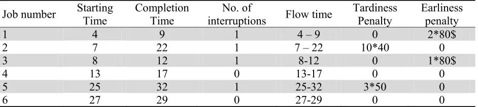
Table 5 presents the solution obtained for each job and it contains the starting and completion time, number of interruptions and flow time. Furthermore, tardiness/earliness penalty imposed by each job is calculated in Table 5.

Table 5

The solution obtained for each job

Job number Starting _Time Completion _Time _{interruptions}No. of Flow time Tardiness _Penalty Earliness _penalty

1 4 9 1 4 – 9 0 2*80$

2 7 22 1 7 – 22 10*40 0

3 8 12 1 8-12 0 1*80$

4 13 17 0 13-17 0 0

5 25 32 1 25-32 3*50 0

6 27 29 0 27-29 0 0

We implement the sensitive analysis of model by increasing the interruption cost of job 3 from 6 to 300. The job schedules, objective function and the solution obtained for each job is presented in Fig 5 and tables 6 and 7, respectively. Increasing in the interruption cost of job 3 causes that model tries to prevent interruption in processing of job 3. As a result, the flow time of jobs 1, 2 and 4 are increased. As we can see, job 3 is processed without any interruption and the flow time of jobs 1, 2 and 4 are increased from 6, 16 and 5 to 10, 17 and 6, respectively. Also the tardiness of job 1, 2 and 4 are increased. By comparing the objective function values presented in Tables 4 and 6, we can understand that in spite of processing job 3 without any interruption, increased flow time of jobs 1 and 2 raise the objective function from 950 to 1222.

M

5 10 15 20

. . .

20 25 30 32 Fig. 5. Job schedules with increased interruption cost

J1 J1 J1 J2 J3 J1 J3 J3 J3 J4 J4 J4 J4 J4 J2 J2 J2

J2 J5 J5 J6 J6 J6

J2 J5 J5 J5

J1

J1 J1 J2 J3 J3 J3 J3 J4 J1 J4 J4 J4 J2

J2

J4 J2

J2 J5 J5 J6 J6 J6

(12)

Table 6

Objective function and its cost components with increased interruption cost

OFV Earliness Tardiness Work-in-process Interruption

1222 80 970 149 23

Table 7

The solution obtained for each job with increased interruption cost

Job number Completion _Time _interruptionNo. of Flow time Tardiness _Penalty Earliness _penalty

1 9 0 6-9 0 0

2 14 1 1-14 2*60$ 0

3 12 1 5-12 0 0

4 19 0 15-19 2*80$ 0

5 29 1 22-29 0 0

6 28 0 26-28 0 1*30$

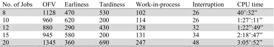
Further to the explained example, we have also solved several numerical examples of different sizes and their results are shown in Table 8.

Table 8

Several numerical examples and related cost components of objective functions

No. of Jobs OFV Earliness Tardiness Work-in-process Interruption CPU time

8 1128 470 530 102 26 40’:32”

10 960 620 200 114 26 1:27’:11”

12 880 290 430 128 32 1:22”:49”

15 945 580 200 131 34 2:18’:47”

20 1345 360 690 247 48 3:05’:52”

6. Conclusions and further research

This paper presented a novel integer nonlinear programming model for the single machine scheduling problem with preemptive jobs in JIT environment to minimize the total tardiness/earliness penalties, interruption penalties and holding costs of all jobs which are work-in-process. The excellent advantage of the proposed model is to incorporate penalties of interruption and work-in-process jobs. The nonlinear formulation of the proposed model was liberalized using an innovative procedure. The performance of the model was illustrated by a numerical example. Sensitive analysis performed on interruption cost illustrated the impact of this feature on the model performance. CPU time required to reach optimal solution for the presented examples shows that obtaining an optimal solution for such hard problems in a reasonable time is computationally intractable.

An attractive future research trend is to investigate the preemptive jobs in JIT with parallel uniform or different machines. Also it would be appropriate to consider the problem studied here with the addition of some other assumptions like sequence dependent setup times. It is also interesting to work on other solution methods like stochastic algorithms and meta-heuristic algorithms to achieve even better results.

Appendix A. The Proof of proposition 1

(13)

(i) Xij > Xij+1. By (10), XPij - XMij > 0. Since this is a minimization problem and the objective

function cost coefficients are strictly positive, XMij = 0 and XPij = Xij - Xij+1 will hold in the

optimal solution.

(ii) Xij < Xij+1. By (10), XPij - XMij < 0. In this case, again with the coefficients of XPij and XMij

being strictly positive, the objective function will ensure that XPij = 0 and thus XMij = Xij+1 -

Xij will hold in the optimal solution.

(iii) Xij = Xij+1. By (10), XPij - XMij = 0. In this case, both XPij = 0 and XMij = 0 will hold in the

optimal solution since their coefficients in the objective function are strictly positive.

Appendix B. The Proof of proposition 2 Consider the following two cases:

(i) Xij .(Ci - j) = 0. Such a situation arises under one of the following three sub-cases:

(a) Xij= 1 and (Ci - j) = 0. ∀i j, ;

(b) Xij= 0 and (Ci - j) > 0. ∀i j, ;

(c) Xij= 0 and (Ci - j) = 0. ∀i j, ;

In all of the three sub-cases given above, the value of Mij = 0, because in these cases, constraint

(11) implies Mij ≥ 0 or -∞ and since Mij has a strictly positive cost coefficient, the minimizing

objective function ensures that Mij = 0.

(ii) Xij .(Ci - j) = (Ci - j) > 0. ∀i j, ;

Such a situation arises when Xij = 1 and (Ci - j) > 0 so, constraint (11) implies Mij ≥ (Ci - j) and

since Mij has a strictly positive cost coefficient, the minimizing objective function ensures that

Mij = (Ci - j).

Appendix C. The Proof of proposition 3

Consider the following two sections:

(i) In term max( _ij. )

j X j , we find the final position of process for job i, thus in constraint (12.2),

when for the final position, for example position j, Xij = 1, then Qij takes value j and for the

following positions which are larger than j, Xijs take value 0, then Qij finally turns value j

which implies the final position of process in constraint (12.2).

(ii) The non-linear constraint (12.2) can be liberalized by the following transformations

1.

ij ij ij

Q ₋ X =R and .j X_ij =F_ij, under the following sets of constraints:

1 (1 ) , ;

ij ij ij

R ≤Q ₋ +A −X ∀i j (12.3)

1 (1 ) , ;

ij ij ij

R ≥Q₋ −A −X ∀i j (12.4)

. , ;

ij ij

R ≤A X ∀i j (12.5)

(14)

(1 ) , ;

ij ij

F ≤ +j A −X ∀i j (12.6)

(1 ) , ;

ij ij

F ≥ −j A −X ∀i j (12.7)

. , ;

ij ij

F ≤ A X ∀i j (12.8)

This section can be shown for each of the two possible cases that can arise. 1. Xij . Qij-1 = Qij-1. ∀i j, ;

Such a situation arises when Xij = 1 so, constraints (12.3) and (12.4) implies Rij ≤Qij-1 and Rij ≥

Qij-1 and ensures that Rij = Qij-1.

2. Xij .Qij-1 = 0. Such a situation arises under one of the following three sub-cases:

(a) Xij= 1 and Qij-1 = 0. ∀i j, ;

(b) Xij= 0 and Qij-1 > 0. ∀i j, ;

(c) Xij= 0 and Qij-1 = 0. ∀i j, ;

In all of the three sub-cases given above, Rij takes the value of 0, because in these cases,

constraint (12.5) implies Rij ≤ 0 and ensures that Rij = 0. Because Rij has not a strictly positive

cost coefficient, the minimizing objective function doesn’t ensures that Rij = 0. Thus, constraint

(12.5) should be added to the mathematical model.

The performance of constraints (12.6) - (12.8) is similar to constraints’ (12.3) and (12.5).

Appendix D. The Proof of proposition 4 Consider the following two sections:

(i) In term _i min (1 _ij)

j

S = ⎡_⎣j+A −X ⎤_⎦, we find the first position of process for job i. In constraint

(13.2), when for the first position, for example position j, Xij = 1, then Bij takes value 1 and

since for the following positions which are larger than j, Bijs takevalue 1, then the summation

of Bijs implies the number of positions where job i is work-in-process. Thus Si returns the

first position number in constraint (13.3).

(ii) The non-linear constraint (13.2) can be liberalized by the following transformation

1.

ij ij ij

B ₋ X =G , under the following sets of constraints:

1 (1 ) , ;

ij ij ij

G ≤B ₋ +A −X ∀i j (13.4)

1 (1 ) , ;

ij ij ij

G ≥B ₋ −A −X ∀i j (13.5)

. , ;

ij ij

G ≤ A X ∀i j (13.6)

Thus, constraints (13.1) - (13.6) should be added to the mathematical model. The performance of constraints (13.4) - (13.6) is similar to constraints’ (12.3) - (12.5).

References

Bector, C.R., Gupta, Y.P., & Gupta, M.C. (1988). Determination of an optimal common due date and optimal sequence in a single machine jobshop. International Journal of Production Research 26,

613–628.

(15)

Davis, J.S., Kanet, J.J. (1993). Single-machine scheduling with early and tardy completion costs.

Naval Research Logistics 40, 85-101.

Esteve, B., Aubijoux, C., Chartier, A., & T’kindt, V. (2006). A recovering beam search algorithm for the single machine Just-in-Time scheduling problem. European Journal of Operational Research

127, 798-813.

Garey, M.R., Tarjan, R.E., & Wilfong, G.T. (1988). One-processor scheduling with symmetric earliness and tardiness penalties. Mathematics of Operations Research 13, 330-348.

Gupta, J.N.D., & Chantaravarapan S. (2008). Single machine group scheduling with family setups to minimize total tardiness. International Journal of Production Research 46, 1707–1722.

Hendel, Y., Runge, N., & Sourd, F. (2009). The one-machine just-in-time scheduling problem with preemption. Discrete Optimization 6, 10-22.

Hendel, Y., & Sourd, F. (2005). The single machine just-in-time scheduling problem with preemptions. In: MISTA 2005: proceedings of the 2nd multidisciplinary international conference on scheduling: theory and applications. p. 140–8.

Hendel, Y., & Sourd, F. (2006). Efficient neighborhood search for the one-machine earliness/tardiness scheduling problem. European Journal of Operational Research 173, 108-119.

Hepdogan, S., Moraga, R., DePuy, G.W., & Whitehouse G.E. (2009). A meta-RaPS for the early/tardy single machine scheduling problem. International Journal of Production Research 47,

1717–1732.

Hoogeveen, J.A., & Van de Velde, S.L. (1996). A branch-and-bound algorithm for single-machine earliness/tardiness scheduling with idle time. INFORMS Journal on Computing 8, 402-412.

Khorshidian, H., Javadian, N., Zandieh, M., Rezaeian, J., & Rahmani, K. (2011). A genetic algorithm for JIT single machine scheduling with preemption and machine idle time. Expert Systems with Applications 38, 7911-7918.

Liao, C.-J., & Cheng, C.-C. (2007). A variable neighborhood search for minimizing single machine

weighted earliness and tardiness with common due date. Computers and Industrial Engineering

52, 404-413.

Luo, X., Chu, Ch., & Wang, Ch. (2006). Some dominance properties for single-machine tardiness problem with sequence-dependent setup times. International Journal of Production Research 44,

3367–3378.

M’Hallah, R. (2007). Minimizing total earliness and tardiness on a single machine using a hybrid heuristic. Computers & Operations Research 34, 3126-3142.

Nandkeolyar, U., Ahmed, M., & Sundararaghavan, P. (1993). Dynamic single-machine-weighted

absolute deviation problem: predictive heuristics and evaluation. International Journal of

Production Research31(6), 1453–1466.

Runge, N., & Sourd, F. (2009). A new model for the preemptive earliness–tardiness scheduling problem. Computers & Operation Research, 36, 2242-2249.

Seidmann, A., Panwalkar, S.S., & Smith, M.L. (1981). Optimal assignment of due dates for a single processor scheduling problem. International Journal of Production Research 19, 393–399.

Shirazi, B., Fazlollahtabar, H., & Sahebjamnia, N. (2010). Minimizing arbitrary earliness/tardiness penalties with common due date in single-machine scheduling problem using a Tabu-Geno-Simulated Annealing. Materials and Manufacturing Processes 25, 515–525.

Sourd, F., & Kedad-Sidhoum, S. (2003). The one-machine scheduling with earliness and tardiness penalties. Journal of Scheduling 6, 533-549.

Sourd, F., & Kedad-Sidhoum, S. (2008). A faster branch-and-bound algorithm for the earliness_tardiness scheduling problem. Journal of Scheduling 11, 49-58.

Szwarc, W., & Mukhopadhyay, S.K. (1955). Optimal timing schedules in earliness/tardiness single machine sequencing. Naval Research Logistics 42, 1109-1114.

Tavakkoli-Moghaddam, R., Moslehi, G., Vasei, M., & Azaron, A. (2005). Optimal scheduling for a single machine to minimize the sum of maximum earliness and tardiness considering idle insert.

(16)

Tavakkoli-Moghaddam, R., Moslehi, G., Vasei, M., & Azaron, A. (2006). A branch-and-bound algorithm for a single machine sequencing to minimize the sum of maximum earliness and tardiness with idle insert. Applied Mathematics and Computation 174, 388-408.

Ventura, J.A., & Weng, M.X. (1994). Single-machine scheduling for minimizing total cost with identical, asymmetrical earliness and tardiness penalties. International Journal of Production Research 32, 2725–2729.

Wan, G., & Yen, B.P.C. (2002). Tabu search for single machine with distinct due windows and weighted earliness/tardiness penalties. European Journal of Operational Research 142, 271-281.