TEST DATA
by
Hannah Luthman
A thesis
submitted in partial fulfillment of the requirements for the degree of Master of Science in Mechanical Engineering
Boise State University
DEFENSE COMMITTEE AND FINAL READING APPROVALS
of the thesis submitted by
Hannah Luthman
Thesis Title: Parameter Estimation for HVAC System Models from Standard Test Data Date of Final Oral Examination: 6 June 2016
The following individuals read and discussed the thesis submitted by Hannah Luthman, and they evaluated her presentation and response to questions during the final oral examination. They found that the student passed the final oral examination.
John F. Gardner, Ph.D. Chair, Supervisory Committee Donald Plumlee, Ph.D. Member, Supervisory Committee Yanliang Zhang, Ph.D. Member, Supervisory Committee
iv
v
The completion of this thesis would not have been possible without the intellectual assistance and encouragement from a number of individuals. First and foremost, I would like to extend a tremendous thank you to my advisor, Dr. John
Gardner, for his continued patience and commitment to me and my research. Dr. Gardner was extremely understanding and supportive when I left school temporarily to enter the workforce. He continued to have weekly meetings with me so that I could attempt to complete my thesis study outside of work. After almost three years of working on my thesis “on the side” he suggested I come back to school full time and complete my Master’s degree. His dedication to me and my research was the push that I needed to make one of the best decisions I could make and come back to school. Not only is Dr. Gardner an exceptional advisor he is also a wonderful person, one who I look up to both professionally and personally. I would also like to thank the remaining members of my supervisory committee, Dr. Don Plumlee and Dr. Yanliang Zhang for their time and direction throughout the finalized stages of this milestone. Kelly Moylan provided me with valuable assistance in ways she will never understand and, for that, I am truly grateful. Her encouragement and support was always there when I had difficulties or questions regarding my professional life.
vii
Nearly all cooling systems, and an increasing proportion of heating systems, utilize the vapor compression cycle (VCC) to provide and remove heat from conditioned spaces. Even though the application of VCC’s throughout the building environment is ubiquitous, effective and accessible models of the performance of these systems remains elusive. Such models could be important tools for VCC designers, building designers and building energy managers as well as those who are attempting to optimize building energy performance through the use of model-based control systems.
Strides have been made in developing lumped parameter models for VCC’s. In spite of these contributions, widespread accessibility and use of VCC performance models has yet to be achieved. This work addresses one of the barriers in applying VCC performance models, the identification of model parameter values required to make performance models useful and accurate. A steady state spreadsheet-based model has been developed which, when combined with standard test data provided by system manufacturers, allows the modeler to identify the salient heat transfer parameters that govern the behavior of the condensers and the evaporators.
Performance data provided by the system manufacturer was used to determine model parameter values. Data used from the test conditions for the determination of these parameters include the evaporating and condensing pressures, the input power, the
viii
geometry. Using an effective heat transfer value allows for the spreadsheet-based model to use a broad spectrum of VCC models despite their potential differences in heat
exchanger design conditions, that is not dependent on the number and spacing of fins or other optimization design criteria.
To validate the concept, the approach was used to identify parameter values for three different air conditioning units with three different sets of performance
specifications. On average the model predicted a heat absorption rate within 1.5% - 3.7% error of what was measured by the manufacturer during testing. This model requires limited sensor information to provide parameters determined under steady state
ix
DEDICATION ... iv
ACKNOWLEDGEMENTS ... v
ABSTRACT ... vii
LIST OF TABLES ... xiii
LIST OF FIGURES ... xiv
LIST OF EQUATIONS ... xv
LIST OF ABBREVIATIONS AND NOMENCLATURE ... xvii
Abbreviations ... xvii
Nomenclature ... xvii
Symbols... xvii
Subscripts ... xviii
CHAPTER ONE: INTRODUCTION ... 1
Energy Efficiency ... 1
VCC Cycle ... 1
CHAPTER TWO: REFRIGERATION CYCLE ... 5
Ideal VCC System... 6
Actual VCC System ... 8
Evaporator ... 9
Compressor ... 10
x
CHAPTER THREE: MOVING BOUNDARY METHOD ... 15
Model Concerns ... 16
Method Description ... 16
Heat Exchangers ... 18
Evaporator ... 19
Condenser ... 21
Compressor ... 22
Flow Restrictor... 23
Interaction of the Component Models ... 24
CHAPTER FOUR: STEADY-STATE COMPONENT MODELING ... 25
Heat Exchangers ... 25
Evaporator ... 30
Condenser ... 30
Mass Balance ... 30
VCC Refrigeration Mass... 31
Mean Void Fraction ... 33
CHAPTER FIVE: PARAMETER DETERMINATION ... 36
Spreadsheet Methodology ... 38
Thermodynamic Add-In... 38
Solver ... 38
Assumptions ... 40
xi
Compressor ... 46
Flow Restrictor... 47
Parameter Result ... 48
CHAPTER SIX: MODEL VALIDATION ... 49
User Input... 49
Outcome ... 50
Results ... 51
Utilized Test Conditions ... 51
New Test Conditions... 52
Replication of Model ... 53
Distribution of Test Conditions ... 56
CHAPTER SEVEN: CONCLUSION ... 59
Research Contributions ... 59
VCC System Designers... 60
Building Designers... 60
Building Energy Managers ... 61
Utility Companies ... 61
Future Research ... 61
REFERENCES ... 64
APPENDIX A ... 68
xii
Mean Void Fraction Derivation ... 72
APPENDIX C ... 76
Parameter Tuning ... 76
APPENDIX D ... 80
xiii
Table 1: Refrigerant Phases ... 9
Table 2: VCC Components Containing Refrigerant Mass ... 31
Table 3: Minimum Required Tests to Determine Parameters ... 42
Table 4: Parameters at Each VCC Unit... 55
Table 5: Final Results of Simulated VCC Units ... 56
xiv
Figure 1: Ideal Vapor Compression Cycle ... 6
Figure 2: Temperature / Entropy Diagram for Ideal Vapor Compression Cycle ... 7
Figure 3: Temperature / Entropy Diagram for Real Vapor Compression Cycle ... 8
Figure 4: Diagram of Thermal Expansion Valve Operation ... 13
Figure 5: Lumped Parameters at the Condenser... 17
Figure 6: Lumped Parameters at the Evaporator ... 17
Figure 7: Information Flow between Systems ... 24
Figure 8: Temperatures Surrounding Heat Exchanger Performance ... 28
Figure 9: Simplification for Heat Transfer Components ... 29
Figure 10: Goodman GPC1436H41 Air Conditioner ... 37
Figure 11: Copeland ZP31K5E-PFV-830 Scroll Compressor ... 46
Figure 12: 0.065 Flow Restrictor... 47
Figure 13: Block Diagram Summarizing Parameter Results ... 48
Figure 14: Process Flow Chart of Model Generation ... 54
xv
Equation 1: Dynamic Model for Evaporator ... 19
Equation 2: Dynamic Model Functions for Evaporator ... 20
Equation 3: Dynamic Model State Variables for Evaporator ... 20
Equation 4: Dynamic Model Input Variables for Evaporator ... 20
Equation 5: Dynamic Model for Condenser ... 21
Equation 6: Dynamic Model Functions for Condenser ... 21
Equation 7: Dynamic Model State Variables for Condenser ... 22
Equation 8: Dynamic Model Input Variables for Condenser ... 22
Equation 9: Flow rate Through Compressor ... 22
Equation 10: Enthalpy without Isentropic Efficiency ... 23
Equation 11: Enthalpy with Isentropic Efficiency ... 23
Equation 12: Flow rate through Flow Restrictor ... 23
Equation 13: Steady State Model for Evaporator ... 26
Equation 14: Steady State Model for Condenser ... 26
Equation 15: Effective Heat Transfer for Superheat Zone - Condenser ... 27
Equation 16: Steady Heat Transfer between Refrigerant and Tube Wall ... 27
Equation 17: Steady Heat Transfer between Tube Wall and Air ... 27
Equation 18: Two-Phase Region - Evaporator ... 30
Equation 19: Superheat Region - Evaporator ... 30
xvi
Equation 22: Subcool Region - Condenser ... 30
Equation 23: Refrigerant Mass of Split System ... 32
Equation 24: Refrigerant Mass of Packaged Unit ... 33
Equation 25: Mean Void Fraction at Evaporator ... 34
Equation 26: Refrigerant Mass at Evaporator ... 34
Equation 27: Mean Void Fraction at Condenser ... 34
Equation 28: Refrigerant Mass at Condenser ... 35
Equation 29: Region Length Relationships within Evaporator ... 43
Equation 30: Percent Error ... 44
Equation 31: Boundary Length Relationships within Condenser ... 45
Equation 32: Original: Heat Transfer between Tube Wall and Air... 69
Equation 33: Modified: Heat Transfer between Tube Wall and Air ... 69
Equation 34: Original: Heat Transfer between Refrigerant and Tube Wall ... 69
Equation 35: Modified: Heat Transfer between Refrigerant and Tube Wall ... 69
Equation 36: Modified: Wall Temperature ... 70
Equation 37: Superheated Flow within the Condenser ... 70
Equation 38: Original: Mean Void Fraction for Evaporator ... 73
Equation 39: Modified: Mean Void Fraction for Evaporator ... 74
Equation 40: Original: Mean Void Fraction for Condenser ... 74
xvii Abbreviations
VCC Vapor Compression Cycle
TX Thermal Expansion
EE Electronic Expansion
Nomenclature
Symbols
𝐴 Area [𝑓𝑡2]
𝐶 Component Coefficient [𝑑𝑖𝑚𝑒𝑛𝑠𝑖𝑜𝑛𝑙𝑒𝑠𝑠]
𝐷 Diameter [𝑓𝑡]
ℎ Refrigerant Enthalpy [𝐵𝑇𝑈
𝑙𝑏𝑚]
𝐿 Total Length [𝑓𝑡]
𝑙 Boundary Length [𝑓𝑡]
𝑀 Mass [𝑙𝑏𝑚]
𝑚̇ Flow rate [𝑙𝑏𝑚
ℎ𝑟]
𝑃 Refrigerant Pressure [𝑙𝑏𝑓
𝑖𝑛2]
𝑄̇ Heat Transfer Rate [𝐵𝑇𝑈
ℎ𝑟]
𝑠 Refrigerant Entropy [ 𝐵𝑇𝑈
𝑙𝑏𝑚∗𝑅]
xviii
𝑊̇ Work [𝐵𝑇𝑈
ℎ𝑟]
𝑥 Refrigerant Quality [𝑑𝑖𝑚𝑒𝑛𝑠𝑖𝑜𝑛𝑙𝑒𝑠𝑠]
𝛼 Convective Heat Transfer Coefficient [𝐵𝑇𝑈
ℎ𝑟∗𝐹]
𝛾̅ Mean Void Fraction [𝑑𝑖𝑚𝑒𝑛𝑠𝑖𝑜𝑛𝑙𝑒𝑠𝑠]
𝜂 Efficiency [𝑑𝑖𝑚𝑒𝑛𝑠𝑖𝑜𝑛𝑙𝑒𝑠𝑠]
𝜈 Refrigerant Specific Volume [𝑓𝑡3
𝑙𝑏𝑚]
Υ Effective Displacement Volume [𝑓𝑡3]
𝜌 Refrigerant Density [𝑙𝑏𝑚
𝑓𝑡3]
𝜔 Compressor Motor Shaft Speed [𝑟𝑎𝑑
ℎ𝑟]
Subscripts
2, 2′, 2′′, 3 Zone Numbers for Condenser
4, 4′, 1 Zone Numbers for Evaporator
4𝑓 Saturated Fluid at State 4
4𝑔 Saturated Vapor at State 4
𝐶 Condenser
𝑐1, 𝑐2, 𝑐3 Superheated, Two-Phase, Subcooled zones in condenser
𝑐𝑖 Inner Tube of Condenser
𝑐𝑜 Condenser Tubing to Ambient Air
𝑐𝑟1, 𝑐𝑟3 Average Values in Superheated, Subcooled Zones of Condenser
xix
𝑒1, 𝑒2 Two-Phase, Superheated zones in evaporator
𝑒𝑎 Temperature of Conditioned Space
𝑒𝑟2 Average Values in Superheated Zone of Evaporator
𝑒𝑖 Inner Tube of Evaporator
𝐻 Total Heat Rejected at the Condenser
𝑖𝑛 Input
𝑘 Compressor
𝐿 Total Heat Absorbed at the Evaporator
𝑜 Outer Diameter of Heat Exchanger Tubing
𝑜𝑎 Outside Air Temperature
𝑠 Entropy
𝑠𝑎𝑡 Two-Phase Region of Evaporator and Condenser
𝑆𝐻 Superheat Region of Evaporator and Condenser
𝑠𝑢𝑏 Subcool Region of Condenser
CHAPTER ONE: INTRODUCTION Energy Efficiency
The worldwide demand for electricity has driven a growing interest in
conservation, renewable generation and energy storage. When it comes to appetites for energy usage, Americans are the most voracious in the world. As a nation, we only represent 5% of the total world’s population yet we consume 20% of the total energy produced (World Population Balance 2001 - 2014). This suggests that if anyone has the ability to improve efficiency it is the American population. As a nation, Americans have become accustomed to luxuries that not everyone enjoys. For example, in 2015 it was found that approximately 87% of American homes and residences utilize an
air-conditioning system of some sort and that percentage continues to increase (Sivak 2015). The main purpose of air conditioning is simply to make the occupant of a building more comfortable during warm weather cycles. It is interesting to note that such a system is highly used and yet the average owner of the system knows nothing about it other than the settings on the thermostat. There are ways in which one can conserve overall energy consumption and improve efficient use of energy while maintaining a level of comfort. However, his is not achievable unless there is an understanding of the system and its functionality.
VCC Cycle
space by use of refrigerant filled tubing (Cengel and Boles 2008). In cooling systems, this refrigerant is used to transfer heat from the air inside a conditioned space to the ambient outside air. Since the first applications in the nineteenth century, great strides have been made in the design and operation of these mechanical refrigeration systems, yet, in order to increase the design efficiency of these units the ability to model their performance must also evolve (Refrigerator 2016). Traditionally, the most practical way of studying the system cycle performance is through mathematical modeling. Standard science and engineering formulas are applied to mathematically describe processes occurring within a given cycle. This is a key first step in simulation and optimization modeling.
Originally, the process for modeling VCC units required reviewing the performance curves of the various components involved in the system. As conditions changed, the ideal operating point was found by locating the intersection of the
appropriate component performance curves. This was a very graphical process requiring a large amount of empirical data for each model and design iteration. Unfortunately, using this approach, there was no ability to get real time results on how the machinery was operating. More recently, with the assistance of computer modeling software,
applications of this method. More recently (McKinley and Alleyne 2008) have expanded upon this research to include a more common heat exchanger design with the inclusion of fins to the condenser and evaporator tubing. This method incorporates the heat
transferred between the refrigerant to the tubing, through the tubing, the tubing to the fins, and the fins to the outside ambient air as well.
Past models have been developed to determine the output of the dynamic system for one specific air conditioner that could be tested in an engineering lab. While this is a step in the right direction, there are shortcomings to these models, specifically their applicability to a variety of air conditioning systems. All of the provided research is only applicable for a specific model of air conditioning unit and requires a rigorous testing program for each new model.
This thesis describes a physics-based model that uses steady state conditions, as can be found in manufacturers’ test data, to determine model parameters that can be used in a variety of dynamic and steady-state models for energy saving estimations. This approach is adaptable to a wide variety of air conditioner specifications and sizes. The model is not dependent on a specific heat exchanger design as it utilizes an effective value that will accommodate current designs as well as future innovations. The model uses empirically driven values measured by the air conditioner manufacturer during testing. This provides values that are not theoretically derived yet do not require extensive testing for the user to facilitate to obtain the parameters required to run the model.
CHAPTER TWO: REFRIGERATION CYCLE
The very first space conditioning system was invented in 1851 by Dr. John Gorrie to reduce diseases, like malaria. His thought was that by keeping patients cool and
comfortable their recovery time would be sped up and the spread of the contagion would be greatly reduced (Lester 2015). The research and development in cooling systems from there was very slow to gain traction. In 1902 Willis Haviland Carrier began the initial design for the modern air conditioner. By the 1920’s air conditioning in public buildings became increasingly popular. This increase in popularity was due to American attendance at the local movie theaters to see their favorite Hollywood stars on the big screen. Again, after many years of scientific development, installment of central air conditioning in an individual’s household substantially increased in the 1970’s (Green 2015). The rapid increase in market penetration of air conditioning systems served to exacerbate the energy crisis of the 1970’s. To assist in the resolution of this crisis, laws were passed to set equipment standards for air conditioners and reduce overall energy consumption. These regulations and design condition requirements have been the basis of the standards that are still in effect today.
uncover the layers involved and the design improvements made they will soon realize that this system is in fact extremely complicated and underappreciated.
Ideal VCC System
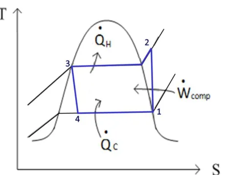
In an ideal system, the refrigerant in a VCC leaves the evaporator as a saturated vapor and immediately enters the compressor, shown as the first state in Figure 1. The saturated vapor is then compressed causing both the temperature and the pressure of the refrigerant to increase. Since the temperature is increased during compression the refrigerant will then be forced into a superheated state at the exit of the compressor and the entrance of the condenser, shown as state two. The ideal cycle assumes isentropic compression.
Figure 1: Ideal Vapor Compression Cycle. Reprinted from Kissock, Kelly. "Energy Efficient Buildings: Chillers." Dayton, OH: Unitversity of Dayton, January 2012.
that the temperature entering the condenser is constant and the same year around because heat rejection rates will change depending on atmospheric temperatures, which change from day to day.
From states three to four, the refrigerant goes through a flow restricting, or throttling, valve, assumed isenthalpic, which will reduce both the temperature and the pressure. The temperature is reduced low enough that it will absorb the excess heat from the conditioned space while in the evaporator where it transitions from state four to state one, thus completing the cycle. As a reversal to the condenser operation, the refrigerant in the evaporator must be low enough to enable heat transfer from the conditioned space to the evaporator. This process is dependent on the set point temperature of the conditioned space and can be changed at any time during operation. A view of the components of a VCC was seen earlier and a thermodynamic graph of this ideal cycle at each refrigerant state can be seen in Figure 2.
Figure 2: Temperature / Entropy Diagram for Ideal Vapor Compression Cycle
is a substantial decrease in temperature due to refrigerant superheat in the first portion of the condenser but the diagram reflects that this temperature reduction happens very quickly and then remains constant across majority of the condenser.
Actual VCC System
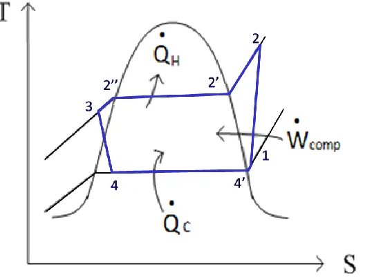
There are safety factors built into mechanical designs to keep the system from failing, and air conditioners are no different. It cannot be stressed enough that the views in Figure 1 and Figure 2 are for an idealized system. A thermodynamic view of a more realistic refrigeration cycle can be seen in Figure 3.
Figure 3: Temperature / Entropy Diagram for Real Vapor Compression Cycle
typically seen in these systems, it is an assumption that is widely used in the research for this thermodynamic process.
For the analysis laid out within this paper the actual VCC system will be employed with reference to the states as shown in Figure 3. When comparing the ideal cycle to the actual cycle there are many additional states within the system that appear. These states and their refrigerant properties are shown below in Table 1.
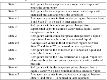
Table 1: Refrigerant Phases
State 1 Refrigerant leaves evaporator as a superheated vapor and enters the compressor
State 2 Refrigerant leaves compressor as a superheated vapor with increased pressure and enters the condenser
State cr1 Average state values in first condenser region; between State 2 and State 2’ (to be used in later equations)
State 2’ Refrigerant within condenser phase changes from
superheated vapor to saturated vapor then a liquid / vapor two-phase combination
State 2’’ Refrigerant within condenser phase changes from a liquid / vapor two-phase combination to a saturated liquid
State cr3 Average state values in third condenser region; between State 2’ and State 2’’ (to be used in later equations)
State 3 Refrigerant leaves the condenser as a subcooled liquid and enters the flow restrictor
State 4 Refrigerant leaves the flow restrictor as a liquid / vapor two-phase combination and enters the evaporator with a reduced pressure
State 4’ Refrigerant within the evaporator phase changes from a liquid / vapor two-phase combination to a saturated vapor State er2 Average state values in second evaporator region; between
State 4’ and State 1 (to be used in later equations)
Evaporator
through phase changes and absorb heat quickly and efficiently. Air conditioners are often designed with a specific refrigerant type in mind. The refrigerant chosen is dependent on environmental considerations, cost, and the ability to optimize the ease of phase change. It is during this phase change within the evaporator that allows for the highest heat absorption rate allowable for the design of the unit.
In the evaporator, the refrigerant enters the evaporator coil immediately after leaving the thermal expansion valve at state four. At this point the refrigerant is in the two-phase region including both vapor and liquid properties. The quality of the mixture defines what portion of the refrigerant is in the liquid state and what portion is in the vapor state. As the refrigerant within the evaporator begins to absorb the heat from the conditioned space more of the liquid evaporates. This process continues and eventually the refrigerant leaves the evaporator as a superheated vapor.
Compressor
In the actual VCC measures are taken to ensure the system is working correctly with no failure. For example, at state one, the temperature is actually pushed into the superheat region by metering the flow into the evaporator. This ensures that the
refrigerant entering the compressor contains no liquid particles. If there is liquid entering the compressor the compressor will not work properly and there will be substantial capital costs to fix or replace that component of the system.
superheated region at a much higher pressure and temperature as it enters the condenser so that the heat can easily be rejected into the outside atmosphere.
Condenser
In contrast to the evaporator, the main purpose for the condenser is to reject the heat absorbed by the evaporator and the compressor work, which was converted to heat, to the atmosphere. Much like the evaporator, the condenser function is highly dependent on the phase change of the refrigerant. Once the compressor discharges the superheated refrigerant to the condenser it begins to reject heat to the atmosphere. Once enough heat is rejected, the refrigerant becomes saturated vapor. Further heat loss transforms the refrigerant into a two-phase mixture of liquid and vapor. The heat is continually being rejected to the atmosphere causing the refrigerant to eventually condense into a liquid. The two-phase portion of the heat exchanger accounts for majority of the heat transfer available to this component of the system. In most cases, the additional capacity beyond this point and the refrigerant continues to reject heat until it leaves the condenser as a subcooled liquid.
Flow Restrictor
As can be expected there are various components in this system that can be modified to improve efficiency and decrease energy consumption. These components tend to come at a cost to the manufacturer so they have the option on deciding what improvements they are willing to incorporate into their model. One of the components that are the easiest to modify is the flow restrictor. Every air conditioning system has a flow restrictor but the complexity of this component may vary. While there are many types of flow restrictors the three most common are the fixed orifice, the electronic expansion valve and the thermal expansion valve.
Fixed Orifice
The fixed orifice design restricts the flow regardless of operating conditions. Due to its simplified nature this is the easiest flow restrictor to compute and model. Because the component is unchanging both the valve coefficient and the area remain constant regardless of operating conditions. This component is the most economical option and is found in most residential air conditioning systems because reliability is often more highly valued than efficiency.
Electronic Expansion Valve
Thermal Expansion Valve
It is most common for commercial air conditioners to utilize a thermal expansion valve, TX valve, to restrict refrigerant flow. A TX valve uses mechanical feedback to regulate the amount of superheat achieved for a variety of operating conditions. A
sensing bulb is fastened to the refrigerant outlet of the evaporator. This bulb is filled with two-phase refrigerant and as the temperature of the system raises the saturation pressure within the sensing bulb increases as well. This pressure acts on a diaphragm inside the valve causing it to open and increase fluid flow to the evaporator and thus reducing the degree of superheat. A pictorial view of this process can be seen in Figure 4.
Figure 4: Diagram of Thermal Expansion Valve Operation. Reprinted from Rasmussen, Bryan Philip. Dynamic Modeling and Advanced Control of Air Conditioning and Refrigeration Systems. Urbana, Illinois: University of Illinois, 2005.
CHAPTER THREE: MOVING BOUNDARY METHOD
In an attempt to improve the ability to model system performance various methods have been established. One of the popular processes for modeling the VCC is the “moving boundary method” which is a type of lumped parameter model with a fixed number of zones that change in length. The complexity of this model was originally presented in (Wedekind and Stoeker 1966) and expanded upon by (Grald and MacArthur 1992) and many others since then. In this method the total length of the heat exchangers are divided into zones containing gas, liquid or mixed phases of the working fluid. This procedure is commonly used because it provides a computationally efficient and effective way of capturing the complexities of the heat exchangers used within the overall system.
Considering most of the air conditioner operation happens within the heat
exchangers of the system, the evaporator and the condenser designs can be intricate. The refrigerant enters these heat exchangers at one thermodynamic state and exits as another. Knowing when these phase changes happen and the lengths of each division is important in understanding the overall efficiency of the system and the overall heat transfer
performance is dependent on the location of these boundaries.
(Bendapudi 2004). Applying the moving boundary method provides greatly reduced computation time because the focus is on a minimum number of zones with variable lengths instead of many zones with fixed lengths.
Model Concerns
One of the concerns with using the moving boundary model is that the model may become singular and fail under certain operating conditions. For example, if a zone within the heat exchanger becomes zero in length, the governing equation set will
become singular which will cause the simulation to fail. Because of this, the applicability of the initial approach of the model can often be considered as both limited and
incomplete (McKinley and Alleyne 2008). Singularities most likely occur during the system start-up and shut-down as well as extreme and sudden changes to operating conditions, which does not often occur during typical operation. In order to avoid this singularity, parameter tuning must be incorporated to better constrain the model during simulation. Additional constraints must be put into place to ensure the refrigerant enters the compressor as a superheated vapor and enters the flow restrictor as a subcooled liquid while under operation. While these design constraints make the system less efficient, they are also ensuring long term usage of the system.
Method Description
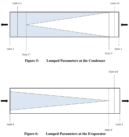
the heat exchangers into a minimum number of divisions. There are three zones within the condenser; the superheated flow between state 2 and state 2’, the two-phase zone between state 2’ and 2’’, and the subcooled zone between state2’’ and state 3 as seen in Figure 5. For the evaporator there are two zones, the two-phase zone between state 4 and state 4’ and the superheated zone between state 4’ and state 1 as seen in Figure 6.
Figure 5: Lumped Parameters at the Condenser
The lengths of these zones change in response to changes in the operating
conditions. This is different than the finite model that has the heat exchangers broken up into dozens of zones with unchanging lengths (Bendapudi 2004). The use of the
minimized number of zones significantly reduces the calculations required to track the refrigerant’s thermodynamic state at every instant during its flow through the heat exchangers yet previous research proves it still provides an accurate overall analysis.
A key simplification used is the assumption that there is not a pressure drop across either of the heat exchangers. The assumption that the pressure drop within the heat exchangers is negligible is incorrect yet universally applied as the pressure drop is extremely minor (Qiao, Aute and Radermacher 2014). In order to understand the effect of the refrigerant properties throughout the entire heat exchanger it is important to calculate the length of each region within each different heat exchanger. The lengths of each region are crucial in determining the total heat transfer rate because both the heat transfer
coefficient and the density of the refrigerant differ from zone to zone. Heat Exchangers
One of the unique attributes of the moving boundary method is that the lengths of each zone are time dependent and integration must be done to track these time varying quantities. Strides have been made in developing lumped parameter models for VCC’s including the groundbreaking work in (X.-D. He 1996) and (McKinley and Alleyne 2008).
dynamics to generate the equations required for his research. The heat transferred from the refrigerant to the tube wall as well as the tube wall to the atmosphere is both
considered. The matrix of equations presented in (X.-D. He 1996) for both the evaporator and the condenser encompasses both energy balance equations as well as mass balance equations due to the nature of the partial derivatives. Since then, research has been done to address concerns with outdated research regarding heat exchanger design, nonlinear air temperature distribution as well as non-circular refrigerant passages (McKinley and Alleyne 2008). The work supports the moving boundary method over a finite volume model but notes the probability of the model becoming singular and failing under atypical operation. This operation includes the possibility that the number of zones within the heat exchangers can be variable and not fixed to three and two for the condenser and
evaporator respectively. Later, the research was taken a step further to understand the basis of operation when the VCC undergoes start-up and shut-down procedures (Li and Alleyne 2010). All of the progress, however, falls back on the foundation that was built in (X.-D. He 1996) including his matrix of equations for both the evaporator and the
condenser which will be presented in the following sections. Evaporator
This paper gets its starting point from the work done in (X.-D. He 1996). He begins with a matrix of partial derivatives and the evaporator dynamic model can be seen in Equation 1.
Equation 1: Dynamic Model for Evaporator
This model is based off of a group of functions as seen in Equation 2 where 𝐱̇𝐄 is the vector of state variables given by Equation 3 and 𝐮E are input variables shown in Equation 4. Expressions of all the elements in the 𝐃𝐄 matrix can be seen in (X.-D. He 1996).
Equation 2: Dynamic Model Functions for Evaporator
𝐟E =
[
ṁihi− ṁihg+ αi1πDiL1(Tw1− Tr1)
ṁohg− ṁoho+ αi2πDiL2(Tw2− Tr2)
ṁi− ṁo
αi1πDi(Tr1− Tw1) + αoπDo(Ta− Tw1)
αi2πDi(Tr2− Tw2) + αoπDo(Ta− Tw2)]
These functions reference inlet and outlet flow rates of the evaporator along with inlet and outlet enthalpies of the various zones. In addition, the heat transfer coefficients of the tubing are needed along with the inner diameter and lengths of the different zones. Lastly, the temperatures of the tube wall, the refrigerant and the conditioned space are included. This group of equations is key and the focus of further analysis later in the thesis.
Equation 3: Dynamic Model State Variables for Evaporator
𝐱E= [Le1 PE heo Tew1 Tew2]T
The state variables of the dynamic model include the length of the two-phase flow zone, the pressure in the evaporator, the enthalpy at the exit and the average wall
temperatures within the two zones.
Equation 4: Dynamic Model Input Variables for Evaporator
Equation 4 shows that the dynamic model of the evaporator takes, as input, the entering and exiting mass flow rate and the entering enthalpy of the heat exchanger. These values are determined by models of the other components of the system. Condenser
Much like the evaporator a basis of study for the condenser operation begins with the work done in (X.-D. He 1996). The matrix of partial derivatives for the condenser dynamic model can be seen in Equation 5.
Equation 5: Dynamic Model for Condenser
𝐃C𝐱̇C = 𝐟C(𝐱C, 𝐮C)
This model is based off of a group of functions as seen in Equation 6 where 𝐱C is the vector of state variables given by Equation 7 and 𝐮C are control variables shown in Equation 8. Expressions of all the elements in the 𝐃C matrix can be seen in (X.-D. He 1996).
Equation 6: Dynamic Model Functions for Condenser
𝐟C =
[
ṁihi− ṁihg+ αi1πDiL1(Tw1− Tr1) ṁohg− ṁohl+ αi2πDiL2(Tw2− Tr2)
ṁohl− ṁoho+ αi3πDiL3(Tw3− Tr3)
ṁi− ṁo
αi1πDi(Tr1− Tw1) + αoπDo(Ta− Tw1) αi2πDi(Tr2− Tw2) + αoπDo(Ta− Tw2) αi3πDi(Tr3− Tw3) + αoπDo(Ta− Tw3)]
transfer coefficients and the inner diameter of the tubing are used along with the temperatures of the tube wall, the refrigerant and the ambient outside air are included.
Equation 7: Dynamic Model State Variables for Condenser
𝐱C= [Lc1 Lc2 PC hco Tcw1 Tcw2 Tcw3]T
The state variables of the dynamic model include the length of the superheat zone and the two-phase flow zone, the pressure at the condenser, the enthalpy at the exit and the average wall temperatures at each of the three zones.
Equation 8: Dynamic Model Input Variables for Condenser
𝐮C= [ṁi hi ṁo ]T
Equation 8 shows that the input for the condenser dynamic model requires the entering and exiting mass flow rate and the entering enthalpy of the heat exchanger. Once again, these values are determined by models of the other components of the system.
Compressor
The compressor design has substantially evolved making it the single most complex component in the VCC. When looking at this feature as a steady operating component, and assuming that the compressor is well insulated, the relationships between compression and flow rate can be determined utilizing the following equation (X.-D. He 1996):
Equation 9: Flow rate Through Compressor
𝑚̇ = 𝜔Υ𝑘 1
𝜐1[1 + 𝐶𝑘− 𝐶𝑘( 𝑃𝐶 𝑃𝐸)
1 2
Equation 9 takes into account the rotating shaft speed of the compressor, 𝜔, as well as a compressor coefficient, 𝐶𝑘, and the effective volume displacement Υ𝑘.
While all other conditions are thermodynamically determined for the compressor analysis, it is important to note that the compression process is an isentropic process and isentropic efficiencies must be taken into account in order to accurately model a system. The relationship between the enthalpies with and without the consideration of isentropic efficiency can be seen in Equation 10 and Equation 11.
Equation 10: Enthalpy without Isentropic Efficiency
ℎ2𝑠 = 𝑓(𝑃2, 𝑠2)
Equation 11: Enthalpy with Isentropic Efficiency
ℎ2 = ℎ1+
ℎ2𝑠− ℎ1 𝜂𝑠
Flow Restrictor
The operation of the flow restrictor, and its relationship to the changing flow rate, can be determined using Equation 12 (X.-D. He 1996). This orifice equation takes into account the valve coefficient, 𝐶𝑣, and the area of the valve opening, 𝐴𝑣; all other values are determined using thermodynamic properties.
Equation 12: Flow rate through Flow Restrictor
𝑚̇ = 𝐶𝑣𝐴𝑣√1
𝜐3∗ (𝑃𝐶− 𝑃𝐸)
an EE valve, the area of the valve is a continually adjustable variable where with the fixed orifice it is a constant value.
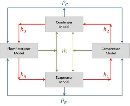
Interaction of the Component Models
Figure 7 reflects how the information flows between the component models to generate the overall analysis of the system. The blue arrows reflect how the pressures are used within each model, the green arrows reflect how the flow rate is used within each model and the red arrows reflect how the enthalpy is used within each model.
CHAPTER FOUR: STEADY-STATE COMPONENT MODELING Heat Exchangers
Typically, the mechanical components of a VCC, the compressor and flow restrictor, are the main focus of research and often times the heat exchangers within the system are overlooked or modeled in an overly simplistic manner. In reality the
evaporator and the condenser are vital components to the overall performance.
Optimizing the design and operation of these pieces will greatly impact the functionality of the whole unit. Reviewing the analysis used in (X.-D. He 1996) for a lumped
parameter model along with other past research, it is common to assume an older design of air conditioner that utilizes smooth circular refrigerant tubes with no fins through the heat exchangers was referenced. Heat exchanger design has significantly developed and is always continuing to make technological advances. One of the major factors in improving heat transfer capabilities and reducing material costs is to add fins to the tubing within the heat exchangers.
While some of the more recent research has utilized a fin design for a heat
incorporate these heat transfer capabilities, there is still a problem with making the model universally adaptable. The problem with previous research is that the information
available is only applicable to a single model and design of air conditioner.
The first step in overcoming this barrier is to create a model with parameters that are simple enough to get from existing data, yet complex enough to model a wide range of systems. At this point, only steady state models are used because manufacturers provided test data was developed under steady state operation and most equipment use is under steady state operation, or very near so. In order to do this, one must take the dynamic model from the literature, as described earlier, and transition to a steady state model by setting the state derivatives to zero. This transition forced the state derivatives to go to zero turning Equation 1 and Equation 5 into Equation 13 and Equation 14 respectively.
Equation 13: Steady State Model for Evaporator
0 = fE(xE, uE)
Equation 14: Steady State Model for Condenser
0 = fC(xC, uC)
Changing to a steady state model allows for parameter determination using manufacturer provided test data, which was also evaluated under steady-state conditions, allowing the model to be utilized for a variety of VCC units. At this point each of the state derivatives with respect to time, in Equation 2 and Equation 6 are set equal to zero. The thermal mass of the tube walls, an essential part of the dynamic model, is not
the overall effect is combined into an effective heat transfer value per unit length. This value encompasses all heat transfer capabilities and has been adapted using a steady state assumption (X.-D. He 1996). Each of these equations utilizes effective heat transfer per unit length values adapted from He’s work as well. As an example, using the
nomenclature as previously stated, the effective heat transfer per unit length for the superheated phase in the condenser can be seen in Equation 15.
Equation 15: Effective Heat Transfer for Superheat Zone - Condenser
𝑈𝑐1 = (𝛼𝑐𝑖1𝜋𝐷𝑐𝑖∗ 𝛼𝑐𝑜𝜋𝐷𝑜) (𝛼𝑐𝑖1𝜋𝐷𝑐𝑖+ 𝛼𝑐𝑜𝜋𝐷𝑜)
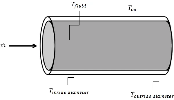
This equation is derived using the steady state versions of the heat transfer equations from the refrigerant to the tube wall and from the tube wall to the outside air.
𝑇𝑐𝑤1 must be solved for in Equation 16 and then the result substituted into Equation 17 as found in (X.-D. He 1996).
Equation 16: Steady Heat Transfer between Refrigerant and Tube Wall
𝑚̇(ℎ2− ℎ2′) + 𝛼𝑐𝑖1𝜋𝐷𝑐𝑖𝑙𝑐1(𝑇𝑐𝑤1− 𝑇𝑐𝑟1) = 0
Equation 17: Steady Heat Transfer between Tube Wall and Air
𝛼𝑖1𝜋𝐷𝑖(𝑇𝑟1− 𝑇𝑤1) + 𝛼𝑜𝜋𝐷𝑜(𝑇𝑎− 𝑇𝑤1) = 0
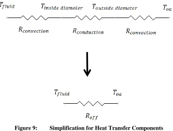
Figure 8: Temperatures Surrounding Heat Exchanger Performance
Figure 9: Simplification for Heat Transfer Components
The effective heat transfer value is a more useful parameter because by making this value a general constant for each refrigerant phase, the model can be utilized for a variety of air conditioners and heat exchanger designs allowing this model to be
replicated time and time again with ease. This approach allows the user the ability to find a parameter that matches the model’s performance to the actual test data. Because of fin geometry and the complexity of the heat transfer in the fins previous models could not grasp this value as simply.
After adapting each equation shown in the matrices presented earlier, the
Evaporator
Equation 18: Two-Phase Region - Evaporator
𝑚̇(ℎ4′ − ℎ4) = 𝑈𝑒1∗ 𝑙𝑒1∗ (𝑇𝑒𝑎− 𝑇4)
Equation 19: Superheat Region - Evaporator
𝑚̇(ℎ1− ℎ4′) = 𝑈𝑒2∗ 𝑙𝑒2∗ (𝑇𝑒𝑎− 𝑇𝑒𝑟2)
Condenser
Equation 20: Superheat Region - Condenser
𝑚̇(ℎ2− ℎ2′) = 𝑈𝑐1∗ 𝑙𝑐1∗ (𝑇𝑐𝑟1− 𝑇𝑜𝑎)
Equation 21: Two-Phase Region - Condenser
𝑚̇(ℎ2′ − ℎ2′′) = 𝑈𝑐2∗ 𝑙𝑐2∗ (𝑇2′ − 𝑇𝑜𝑎)
Equation 22: Subcool Region - Condenser
𝑚̇(ℎ2′′− ℎ3) = 𝑈𝑐3∗ 𝑙𝑐3∗ (𝑇𝑐𝑟3− 𝑇𝑜𝑎)
Utilizing a constant effective heat transfer coefficient for each region that incorporates all aspects of allowable heat transfer provides a unique approach to
identifying censorious parameters required for an accurate VCC model. This framework along with limited sensor information can provide a dynamic model to assist in design, control and operation of traditional VCC systems.
Mass Balance
with unique dynamic states for the mass in the evaporator and the condenser, but those relationships became trivial in the steady state case. Instead, the steady state model will enforce the constraint that the total mass of refrigerant is unchanged under various operating conditions. The mass of a VCC needs to incorporate all applicable components within the system where refrigerant can be located and contribute to the overall
refrigerant mass. This view has been adopted for the model as laid out in this paper, but considering the refrigerant goes through phase changes at different operating conditions the mass in these components will be dependent on time and operating conditions. VCC Refrigeration Mass
Refrigerant mass distribution is dependent on the specific air conditioning unit. While there are four main elements to every VCC, additional mechanisms can be added or modified to increase the efficiency or production of the unit. These additional
components often times include some type of refrigerant mass that needs to be accounted for in the total mass migration of the system. The applicable components for a complex VCC containing refrigerant mass are shown inTable 2.
Table 2: VCC Components Containing Refrigerant Mass
Evaporator The mass within the evaporator is dependent on the tube’s inner diameter, overall tube length and thermodynamic state of the refrigerant
Accumulator
The accumulator is attached to the evaporator outlet to ensure that only vapor is entering the compressor. If the system is running properly and going into superheat all the refrigerant entering the accumulator should be superheated vapor but there could be a small fraction of liquid refrigerant as well that would need to be calculated for in the mass Compressor The mass of the refrigerant at the compressor is minimal but
will still be dependent on the size and specification of the compressor and may need to be considered
Liquid Tube The liquid tubing is the refrigerant between the condenser outlet and the flow restrictor inlet
Additional Piping
Often times in split systems the condenser is located outside and the evaporator supplying the building is located inside. In this case, there are refrigerant lines that run from the outside to the inside and vice versa. The following lengths and tube’s inner diameter need to be considered when accounting for refrigerant mass throughout the migration process:
o Compressor to condenser o Flow restrictor to the evaporator o Evaporator to the accumulator o Accumulator to compressor
Flow Restrictor The mass of the refrigerant within the flow restrictor will be dependent on the type of flow restrictor used
Miscellaneous
Any additional components added to the system
When each of these pieces of equipment is taken into account the mass balance becomes what is seen in Equation 23.
Equation 23: Refrigerant Mass of Split System
𝑀𝑡𝑜𝑡𝑎𝑙 = 𝑀𝐸𝑣𝑎𝑝𝑜𝑟𝑎𝑡𝑜𝑟+ 𝑀𝐴𝑐𝑐𝑢𝑚𝑢𝑙𝑎𝑡𝑜𝑟+ 𝑀𝑃𝑖𝑝𝑖𝑛𝑔+ 𝑀𝐶𝑜𝑚𝑝𝑟𝑒𝑠𝑠𝑜𝑟+ 𝑀𝐶𝑜𝑛𝑑𝑛𝑒𝑠𝑒𝑟
+ 𝑀𝐿𝑖𝑞𝑢𝑖𝑑 𝐿𝑖𝑛𝑒+ 𝑀𝐹𝑙𝑜𝑤 𝑅𝑒𝑠𝑡𝑟𝑖𝑐𝑡𝑜𝑟
refrigerant mass within is negligible. When a fixed orifice is used no mass is being held within the valve so that mass can be removed from the calculation as well. Understanding this, the mass balance equation is easily manipulated and simplified to meet the needs of this analysis; Equation 23 simply becomes Equation 24.
Equation 24: Refrigerant Mass of Packaged Unit
𝑀𝑡𝑜𝑡𝑎𝑙 = 𝑀𝐸𝑣𝑎𝑝𝑜𝑟𝑎𝑡𝑜𝑟 + 𝑀𝐶𝑜𝑛𝑑𝑛𝑒𝑠𝑒𝑟
Mean Void Fraction
In determining the mass migration through a refrigeration system it is common to assume that the enthalpy has a linear profile along the regions making the mass inside readily evaluated. This is why the information within the single-phase regions,
superheated and subcooled, are calculated using the arithmetic average between the two states and the associated length of the region. However, when looking at the two-phase flow within the heat exchangers a more sophisticated approach is required. A mean void fraction model can be applied to calculate the mass within the two-phase flow portion of the heat exchangers (Beck and Wedekind 1981).
As with the length of the moving boundaries, the mean void fraction will also vary depending on time and various conditions that will affect the system. Reviewing the previous work done on the mean void fraction and integrating it into this system
Equation 25 - Equation 28 have been determined to reflect the mean void fraction relationships in both the evaporator and the condenser and their contribution to the total mass calculation. These equations were formed applying the Zivi void fraction
correlation (G.L. Wedekind 1976). For a full derivation of this equation please see Appendix B.
Evaporator
Equation 25: Mean Void Fraction at Evaporator
𝛾̅𝐸 = 1
(1 − (𝜐𝜐4
4′) 2 3
) +
(𝜐𝜐4
4′) 2 3
(1 − 𝑥4) (1 − (𝜐𝜐4 4′)
2 3
)
2∗ 𝑙𝑛 [(
𝜐4 𝜐4′)
2 3
+ (1 − (𝜐4 𝜐4′)
2 3
) ∗ 𝑥4]
Equation 26: Refrigerant Mass at Evaporator
𝑀𝐸 =
𝜋𝐷𝑒𝑖2 4 [𝑙𝑒1(
𝛾̅𝐸 𝜐4𝑔
+1 − 𝛾̅𝐸 𝜐4𝑓
) + 𝑙𝑒2 𝜐𝑒𝑟2
]
Condenser
Equation 27: Mean Void Fraction at Condenser
𝛾̅𝐶= 1
(1 − (𝜐𝜐2′′
2′) 2 3
) +
(𝜐𝜐2′′
2′) 2 3
(1 − (𝜐2′′
𝜐2′)
2 3
)
2∗ 𝑙𝑛 [(
𝜐2′′ 𝜐2′)
2 3
Equation 28: Refrigerant Mass at Condenser
𝑀𝐶 = 𝜋𝐷𝑐𝑖
2
4 [ 𝑙𝑐1
𝜐𝑐𝑟1+ 𝑙𝑐2( 𝛾̅𝐶
𝜐2′+
1 − 𝛾̅𝐶
𝜐2′′ ) + 𝑙𝑐3
𝜐𝑐𝑟3]
Now that the mean void fraction is determined in values that can be inferred from the initial input they can be used to determine the overall mass of the system that is within the evaporator and the condenser.
It is important to note that although the mean void fraction calculated is helpful in acquiring an accurate model, this value is constantly changing. An important
simplification to the mean void fraction study is that the time dependence is neglected. Not only is this value changing in different operating conditions it is also changing throughout the two-phase section of both the evaporator and the condenser. Using a single average value that does not incorporate the time-variance, however, does not cause major impact on the overall system (Beck and Wedekind 1981).
As mentioned earlier, there can be additional components added to the VCC to make the unit more efficient and avoid failure. One of these components is the
CHAPTER FIVE: PARAMETER DETERMINATION
The specific model used to demonstrate this approach was the Goodman PC1436H41 as seen in Figure 10. The model was a 36,000 BTU/hr (3 ton) residential unit that, due to its size, would be applicable to many homeowners. The manufacturers website had most of the required information for the model. If any additional information or clarification was needed a manufacturer representative was contacted to obtain this information or clarity. Once all of the testing data and information on the system was acquired the analysis could proceed. The parameters below are required to be known from the manufacturer’s documentation to run the analysis on the test conditions and utilize the overall model. Where a test variable corresponds to a variable in the model, the variable name is listed:
Suction Pressure, 𝑃𝐸
Discharge Pressure, 𝑃𝐶
Indoor Set Point Temperature, 𝑇𝑒𝑎
Outdoor Ambient Temperature, 𝑇𝑜𝑎
Refrigerant Type
Total Compressor Work, 𝑊̇𝑖𝑛
Degrees of Superheat Degrees of Subcool Compressor Speed, 𝜔
Flow Restrictor Area (only if fixed orifice), 𝐴𝑣
Charge of System, 𝑀𝑡𝑜𝑡𝑎𝑙 Heat Absorption Rate
Once the above information was acquired an operating condition was selected from the test data. A thermodynamic analysis was done to get all the states as listed in Table 1 earlier in the thesis. It is at this point that the refrigerant load was used to back out the mass flow rate for that test condition. The remaining data was used to determine the remaining parameter values and minimize the error within the model.
The documentation received from the manufacturer had all the required information for four different tests using various outdoor ambient temperatures at the same set point temperature. There were three different set point temperatures for these ambient conditions allowing for twelve uniquely tested data points to be used in various examinations to solve for the required parameters. The twelve different test conditions were built in various worksheets within a single Excel document and all the required data was determined for each one. A view of these simulated spreadsheets can be seen in Appendix D.
Spreadsheet Methodology
Thermodynamic Add-In
In order to utilize the spreadsheet based analysis an add-in was required to be downloaded for Microsoft Excel. For this analysis a free download offered by University of Alabama was used (Excel in Mechanical Engineering n.d.). This add-in includes psychometric functions and thermodynamic properties for the following refrigerants: R407C, R410A, R22 and R134a. The VCC model used for this research requires R-410a refrigerant, which is a blended refrigerant common for residential air conditioners and supported by the Excel add-in. This downloaded feature along with Excel’s provided
Solver add-in is all that is needed to replicate the model. Solver
In general, the main purpose of Solver is to find a solution that minimizes or maximizes an objective cell value while satisfying a number of constraints that could be placed on the system. The kind of solution one can expect and computation time depends on three characteristics of the model (Frontline Solvers 2016):
1. The size of the model
a. Including number of variables, constraints and formulas 2. Complexity of mathematical relationships between objective cell and
constraints
a. Nonlinear vs. linear
3. Use of integer versus variables within the model
Using Excel for this model pushes the limits of its capabilities; yet, the model is still accurate when compared against the results of other models in past research using a more sophisticated modeling software program. Once the constraints and the objective cell were determined Solver was ready to be run. To speed up the process the GRG Nonlinear setting in Solver was used. This is a generalized reduced gradient (GRG) algorithm used for optimizing a range of nonlinear problems. It employs an iterative numerical method that involves adjusting trial values for the adjustable cells and
reviewing the results of the objective cell. When multiple values are entered, as with this analysis, partial derivatives and gradients assist in measuring the rate of change
(Microsoft Support 2016).
starting point in the computation. In order to have the analysis run properly initial conditions had to be placed as initial “stand in” values for what was to be determined. The initial assumptions were determined by using relationships seen within the test conditions and can be seen in Appendix C. The second thing to ensure the accuracy of Excel’s Solver was that in some cases the simulation needed to be ran more than once. At most the simulation needed to be run three times, each time providing Solver with more accurate initial conditions.
Assumptions
In both determining the required parameters as well as running the full analysis an array of assumptions were considered. A comprehensive list of these assumptions is shown below:
No pressure drop across heat exchangers
No temperature drop between State 4 and State 4’ No temperature drop between State 2’ and State 2’’ Consistent ambient air temperature across the condenser Constant mean void fraction calculations
85% Isentropic efficiency
No refrigerant mass in the compressor, flow restrictor, and additional tubing Information from manufacturer was detailed and accurate
Solving for Parameters
One of the barriers in applying VCC performance models is the identification of parameter values required to make these models useful. In order to have a model that accurately depicts how the air conditioner is performing various parameters need to be solved for and utilized.
There are a total of eight nonlinear equations which can be used with Excel’s
Solver to identify the parameter values which minimize the errors in previous equations (Equation 9, Equation 12, Equation 18, Equation 19, Equation 20, Equation 21, Equation 22, and Equation 24). Using these equations there are, in total, ten model parameters to be identified. These parameters are listed below:
o Heat Transfer Coefficient for each Region (𝑈𝑒1, 𝑈𝑒2, 𝑈𝑐1, 𝑈𝑐2, 𝑎𝑛𝑑 𝑈𝑐3) o Total Length of Tubing within Evaporator (𝐿𝐸)
o Total Length of Tubing within Condenser (𝐿𝐶)
o Compressor Displacement Volume (Υ𝑘)
o Compressor Coefficient (𝐶𝑘) o Valve Coefficient (𝐶𝑣)
1 Test Condition 15 Unknowns 8 Equations
2 Test Conditions 20 Unknowns 16 Equations
3 Test Conditions 25 Unknowns 24 Equations
4 Test Conditions 30 Unknowns 32 Equations
5 Test Conditions 35 Unknowns 40 Equations
… … …
12 Test Conditions 70 Unknowns 96 Equations
Mass Balance
Since the mass migration of the system are directly related to the region lengths in both the evaporator and the condenser, it is important to solve for these lengths and the mass balance simultaneously. One analysis must be done to ensure that the total length of the tubing and the specific zone lengths mesh appropriately with the mass migration throughout the system. When the analysis is run simultaneously the total tubing length of the evaporator and the condenser can be found. Along with this are the specific lengths of each region in the heat exchangers and their associated heat transfer values per unit length.
Overall Lengths and Mass
In order to solve for the mass at the evaporator and the condenser the mean void fractions from the test conditions was needed as well as the total lengths of the evaporator and the condenser tubing and the specific lengths of each zone within the heat
To determine the unknowns, Solver was used to run an analysis with the twelve test conditions to find the best solution for the various zone lengths and total tubing lengths to satisfy the mass balance equation under specifically determined constraints.
Evaporator
For the evaporator analysis the effective heat transfer per unit length needs to be determined for both the two-phase region and the superheat region. Along with the refrigerant load, as reported in the test conditions, a thermodynamic analysis was done at each test condition to determine the appropriate properties required to successfully compute the region energy balance equations, Equation 18 and Equation 19. An analysis was done comparing the results of the calculated heat absorption rates in both regions using the effective heat transfers against the test condition results. Excel Solver was directed to change the value of one common 𝑈𝑒1 and 𝑈𝑒2 and different 𝑙𝑒1 values for each of the twelve data points. The length of the superheat zone was automatically solved for using the relationship as seen in Equation 29 which is easily done considering the total length of the evaporator has been predetermined when confirming an appropriate mass balance.
Equation 29: Region Length Relationships within Evaporator
𝑙𝑒2 = 𝐿𝐸 − 𝑙𝑒1
The final result provided an analysis with varying zone lengths, as predicted, but a common 𝑈𝑒1 and 𝑈𝑒2 that can be used as parameters in the more evolved model.
which move to accommodate the required heat absorption. The effective heat transfer values are, essentially, an average value across each region it is safe to assume that the heat transfer characteristics will remain largely constant across each region.
There are three different error calculations within the evaporator model; the error associated with heat absorption in the two-phase region, the superheated region and the overall heat absorption in the evaporator. To calculate error throughout this model Equation 30 was employed. Each test condition had two parameters to review, the
parameter directly measured from the test conditions and thermodynamic analysis and the parameter as computed using previous equations. In the case of the evaporator, both 𝑈𝑒1
and 𝑈𝑒2 were solved for simultaneously in order to reduce the overall error associated with the evaporator calculations. When comparing the calculated heat absorbed in the superheated region using the determined 𝑈𝑒2 and Equation 19 there was a high
percentage error against what the test conditions and thermodynamic analysis measured. This error was most notable when paralleled against the percent error within the two-phase region; on average the superheated region had a 20-30% higher error. However, at most the superheated region only contributed 10% of the overall heat transfer required within the evaporator. Since this accounted for such a small portion of the overall heat transfer, the overall error of heat absorption was very minimal. When comparing the values predicted using the effective heat transfer against the values measured during testing, there was a resulting error ranging from 0.06% error to 3.35% error.
Equation 30: Percent Error
Condenser
For the condenser analysis the effective heat transfer per unit length needs to be determined for the three different regions; superheated region, two-phase region and subcooled region. Along with the heat rejection required, as reported in the test
conditions, a thermodynamic analysis was done at each test condition to determine the appropriate properties required to successfully compute the region energy balance equations, Equation 20, Equation 21, and Equation 22. An analysis was done comparing the results of the calculated heat rejection rates in all regions using the effective heat transfers against the test condition results. Excel Solver was directed to change the value of one common 𝑈𝑐1 , 𝑈𝑐2 and 𝑈𝑐3 while allowing 𝑙𝑐1 and 𝑙𝑐2 values to be different for each of the twelve data points. The length of the subcool region was automatically solved for using the relationship as seen in Equation 31 which is easily done considering the total length has been predetermined.
Equation 31: Boundary Length Relationships within Condenser
𝑙𝑐3= 𝐿𝐶− (𝑙𝑐1+ 𝑙𝑐2)
There are four different error calculations within the condenser model; the error associated with heat rejected in the superheated region, the two-phase region, the subcooled region and the overall heat rejected in the condenser. In the case of the
the regions as calculated versus measured, there resulted in various concerns. Most of these concerns fell within the subcool equation but the heat rejection required during this region only contributed 6% at most to the total heat rejection required. The overall percent error ranged from 0.96% to 16.22%.
Compressor
The compressor analysis is straight forward in solving for the unknown parameters essential to the model. The speed of the compressor was given from the manufacturer’s provided information and, for testing purposes, the scroll compressor used as seen in Figure 11, operated at a speed of 1800 RPM. Using this added knowledge along with other test conditioned data all but two parameters were known.
Figure 11: Copeland ZP31K5E-PFV-830 Scroll Compressor
Equation 9, and the flow rate under testing conditions the error ranged from 0.08% to 2.96%.
Flow Restrictor
Similar to the compressor, the flow restrictor analysis was straightforward in determining the unknown parameter. The Goodman air conditioning unit used in this analysis has a fixed orifice flow restrictor which made the results more consistent and predictable because the opening area of the valve was constant. Looking at the flow rate relationship at the flow restrictor, Equation 12, it is clear that, in this case, the only missing parameter is the valve coefficient (X.-D. He 1996).
Figure 12: 0.065 Flow Restrictor
there the opening area could be determined and the remaining values to accommodate Equation 12 can be found under the test conditions.
The resulting valve coefficient for this model was 0.6719 which validates the initial assumption because it was close yet a bit more efficient, like the design reflects. Using the error equation to compare the flow rate computed at the flow restricting valve to the flow rate measured under test conditions this value resulted in an error ranging from 0.0% to 6.8%.
Parameter Result
To conclude this section, all parameters needed to run the final model were determined using information provided within the manufacturers test conditions. Figure 13 summarizes all the information needed and all the parameters that were determined.