D E B A T E
Open Access
Significance testing as perverse probabilistic
reasoning
M Brandon Westover
1*, Kenneth D Westover
2, Matt T Bianchi
1Abstract
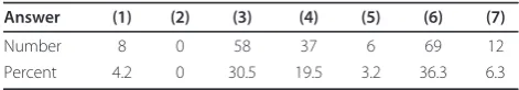
Truth claims in the medical literature rely heavily on statistical significance testing. Unfortunately, most physicians misunderstand the underlying probabilistic logic of significance tests and consequently often misinterpret their results. This near-universal
misunderstanding is highlighted by means of a simple quiz which we administered to 246 physicians at two major academic hospitals, on which the proportion of incorrect responses exceeded 90%. A solid
understanding of the fundamental concepts of probability theory is becoming essential to the rational interpretation of medical information. This essay provides a technically sound review of these concepts that is accessible to a medical audience. We also briefly review the debate in the cognitive sciences regarding physicians’aptitude for probabilistic inference.
Background
Medicine is a science of uncertainty and an art of probability. - Sir William Osler [1]
While probabilistic considerations have always been fundamental to medical reasoning, formal probabilistic arguments have only become ubiquitous in the medical literature in recent decades [2,3]. Meanwhile, many have voiced concerns that physicians generally misunderstand probabilistic concepts, with potential serious negative implications for the quality of medical science and ulti-mately public health [3-12]. This problem has been demonstrated previously by surveys similar to the fol-lowing quiz [13], which we administered to a group of 246 physicians at three major US teaching hospitals (Barnes Jewish Hospital, Brigham and Women’s Hospi-tal, and Massachusetts General Hospital). The reader is
likewise invited to answer before proceeding.
Consider a typical medical research study, for exam-ple designed to test the efficacy of a drug, in which a null hypothesisH0 (’no effect’) is tested against an
alternative hypothesisH1 (’some effect’). Suppose
that the study results pass a test of statistical signifi-cance (that isP-value <0.05) in favor ofH1. What
has been shown? 1.H0is false.
2.H1is true.
3.H0is probably false.
4.H1is probably true.
5. Both (1) and (2). 6. Both (3) and (4). 7. None of the above.
The answer profile for our participants is shown in Table 1. This essay is for readers who, like 93% of our respondents, did not confidently select the correct answer, (7), ‘None of the above’. We hasten to assure the reader that this is not a trick question. Rather, it is a matter of elementary probabilistic logic. As will be clear by the end of this essay answers (1) to (6) involve‘ leap-ing to conclusions’, in violation of the basic law of prob-abilistic inference, Bayes’ rule. We will see that Bayes’ rule is an essential principle governing all reasoning in the face of uncertainty. Moreover, understanding Bayes’ rule serves as a potent prophylaxis against statistical fal-lacies such as those underlying the apparent plausibility of the six erroneous answers in this little quiz.
Despite its central place in the theory of probabilistic inference, Bayes’rule has been largely displaced in the practice of quantitative medical reasoning (and indeed in the biological and social sciences generally) by a statisti-cal procedure known as‘significance testing’. While sig-nificance testing can, when properly understood, be seen as an internally coherent aid to scientific data analysis [14], it is usually misunderstood as a way to bypass Bayes’ rule, which we shall see is a perversion of probabilistic
* Correspondence: [email protected]
1
Department of Neurology, Massachusetts General Hospital, Harvard Medical School, Boston, MA, USA
Full list of author information is available at the end of the article
reasoning. Embarrassingly, fallacious uses of significance testing continue to flourish despite being under constant criticism in the statistical literature since its inception in the 1960 s [5,13,15-17]. The reasons for this state of affairs derive from a complex web of social and philosophical fac-tors. However, we believe a more immediate barrier to physicians understanding probability theory is the lack of adequate literature explaining the subject in a way that physicians can relate to. Therefore, we have written this essay with three aims in mind. The first aim, addressed in ‘Discussion, Part I’, is to explain the basic concepts of probability theory to physicians, and in particular to pro-vide a detailed account of the ‘origin’, mechanics, and meaning of Bayes’rule. The second aim, covered in‘ Dis-cussion, Part II’, is to provide an accurate technical expla-nation of the two ingredients of significance testing: binary hypothesis testing andP-values. Finally, we aim to show how understanding Bayes’rule protects against common errors of statistical reasoning, such as those involved in choosing the wrong answers to our introductory quiz.
Discussion, Part I: probability in medicine Reasoning under uncertainty
They say that Understanding ought to work by the rules of right reason. These rules are, or ought to be, contained in Logic; but the actual science of logic is conversant at present only with things either certain, impossible, or entirely doubtful, none of which (for-tunately) we have to reason on. Therefore the true logic for this world is the calculus of Probabilities, which takes account of the magnitude of the prob-ability which is, or ought to be, in a reasonable man’s mind. - James Clerk Maxwell [18]
The inadequacy of deductive logic
Since Aristotle the mainstream Western view has been that rationality means reasoning according to the rules of deductive logic [19,20]. The basic building block of deductive logic is the syllogism, for example:
if is true, then is true. is true.
is true.
A B
A B
∴
Or, similarly:
if is true, then is true. is false.
is false.
A B
B A
∴
These logical forms play a role in straightforward medical diagnostic scenarios like the following:
• 75 year old man with fever, productive cough, chest x-ray showing consolidation of the right upper lobe, sputum culture positive for gram positive cocci in clusters.
Diagnosis: Pneumonia.
•50 year old previously healthy man with sudden onset painful arthritis of the MTP joint of his right great toe, arthrocentesis positive for needle-shaped, negatively birefringent crystals.
Diagnosis: Gout.
The reasoning required to make these diagnoses is essentially syllogistic, that is a matter of checking that the definitions of the disorders are satisfied, then draw-ing the inevitable conclusion.
However, medical reasoning frequently requires going beyond syllogistic reasoning. For example, consider the following argument type:
if is true, then is true. is true.
becomes more plausible.
A B
B A
∴
Of course, given the premise (A⇒ B), the truth of B does not, strictly speaking, imply the truth of A, hence the use of the term‘plausible’ to denote an implication that falls short of certitude. Arguments of this kind, which have been aptly called‘weak syllogisms’ [21], are indispensable in everyday medical reasoning. For exam-ple, it is reasonable to assert that patients with appendi-citis will have abdominal pain, and we accept abdominal pain as grounds for suspecting appendicitis, though logi-cally there are numerous other possible explanations for abdominal pain. In a similar vein, consider these addi-tional typical case vignettes and possible diagnoses:
•45 year old homeless alcoholic man brought in by police with confusion, disorderly behavior, and breath smelling of alcohol. Diagnosis: Ethanol intoxication.
•75 year old nursing home resident with known heart failure presents with confusion and shortness of breath. Physical examination reveals rales, 3+ lower extremity pitting edema, labored breathing. Diagnosis: CHF exacerbation.
•55 year old male presents to ED with acute onset substernal chest pain. Diagnosis: Gastric reflux.
Most physicians quickly assign rough degrees of plausi-bility to these diagnoses. However, in these cases it is rea-sonable to entertain alternative diagnoses, for example in
Table 1 Quiz answer profile
Answer (1) (2) (3) (4) (5) (6) (7)
Number 8 0 58 37 6 69 12
the first case other intoxicants, or meningitis; and in the second case pulmonary embolus, pneumonia, or myocar-dial infarction. In the third case the stated diagnosis is only weakly plausible, and most physicians would doubt it at least until other possibilities (for example myocardial ischemia) are ruled out. In each case, there is insufficient information to make a certain (that is logically deductive) diagnosis; nevertheless, we are accustomed to making judgements of plausibility.
Stepping back once more, we can add to the list of argument types frequently needed in medical reasoning the following additional examples of even weaker ‘weak syllogisms’:
If is true, then becomes more plausible. is true.
becomes more p
A B
B A
∴ llaussible.
and
If is true, then becomes more plausible. is plausible.
becomes
A B
B A
∴ mmore plaussible.
As in syllogistic reasoning, weak syllogistic reasoning combines prior knowledge (for example knowledge of medicine and clinical experience) with new data (for example from seeing patients, lab tests, or new litera-ture), but the knowledge, data, and conclusions involved lack the certainty required for deductive logical reason-ing. The practice of formulating differential diagnoses, and the fact that physicians do not routinely test for every possibility in the differential, shows that physicians do in fact routinely assign degrees of plausibility. The same can be said of most situations in everyday life, in which the ability to judge which possibilities to ignore, which to entertain, and how much plausibility to assign to each constitute ‘common sense’. We now explore the rules that govern quantitative reasoning under uncertainty.
Cox’s theorem and the laws of plausible reasoning There is only one consistent model of common sense. - ET Jaynes [21]
How might one go about making the ‘weak syllo-gisms’, introduced above, into precise quantitative state-ments? Let us attempt to replace the loose statement that‘Abecomes more plausible in light ofB’, with a for-mula telling us how plausible Ahas become. For this purpose, let us denote byAandBthe propositions ‘Ais true’ and ‘B is true’. We assume that we have already assigned an ‘a priori’ value to the plausibility of A,
denoted ( )A . We wish to quantify how much more plausibleAbecomes once we learn the additional infor-mation given in the premises, comprising the plausibility ofB, denoted ( )B , and the plausibility ofBwhenAis
true, ( | )B A . We focus on the third and‘weakest’ syl-logism, of which the other weak syllogisms are special cases. A quantitative re-writing of this statement takes the following form:
The plausibility of without regard to is equal to The plaus
A( B) ( ).A
iibility of without regard to is equal to The plausibility
B( A) ( ).B
o
of when is true is equal to The plausibility of when is
B A B A
A B
( | ).
∴ ttrue is equal to( | ).A B
From this it is apparent that what we are seeking is a formula that gives the strength of the conclusion as a function, f, of the quantities involved in the premises, that is an equation of the form:
( | )A B = f( ( ), ( ), ( | )). A B B A
RT Cox (1898-1991) [22] and ET Jaynes (1922-1998) [23] were able to prove mathematically that the only possible formula of this form suitable for measuring plausibilities was in fact:
Pr A B Pr B A Pr A
Pr B
( | ) ( | ) ( )
( ) ,
=
where the numbers denoted by Prrepresent probabil-ities, subject to the basic laws of probability theory, which are:
•0≤Pr(A)≤1,
•Pr(A) = 0 whenAis known to be false, •Pr(A) = 1 whenAis known to be true, • Pr A( )+Pr A( )=1,
• Pr B( )=Pr B A( , )+Pr B A( , )
In the rest of the paper, we will use the more com-mon form for Bayes’ rule, which is derived from the form given above by simple substitutions using the basic relations of probability just cited:
Pr A B Pr B A Pr A
Pr A Pr B A Pr A Pr B A
( | ) ( | ) ( )
( ) ( | ) ( ) ( | ). =
+
This form is useful in that it makes explicit the fact that Bayes’rule involves three distinct ingredients, namelyPr (A), (and its converse Pr A( )= −1 Pr A( )),Pr(B|A), and
Pr B A( | ). The meanings of these ingredients will become clear in the next section.
We pause before proceeding to comment on our focus in this essay on simple applications of Bayes’rule. Our aim is to explain the basic concepts governing probabilis-tic inference, a goal we believe is best served by using very simple applications of Bayes’rule to evaluating mutually exclusive truth claims (that is‘binary hypoth-eses’). We hasten to add that binary hypothesis compari-son is not necessarily always the best approach. For instance, in the quiz beginning this essay, rather than pit-tingH0(’no effect’) against hypothesisH1(’some effect’),
it may be more informative to consider a range of possi-ble value for the strength of the effect, and to compute a probability distribution over this range of possible effect sizes, from which we could also‘read off’the credibility of the hypothesis that the effect size is equal to or close to zero. The perils of inappropriate uses of binary hypothesis testing, and alternative Bayesian methods for assessing hypotheses, are discussed at length in several good books and articles, for example [25,26].
Indeed, much real-world medical reasoning cannot be naturally reduced to evaluating simple‘true/false’ judge-ments, but requires instead the simultaneous analysis of multiple data variables, which often take on multiple or a continuous range of values (not just binary). There are frequently not just two but many competing interpreta-tions of medical data. Moreover, we are often more interested in inferring the magnitude of a quantity or strength of an effect rather than simply whether a state-ment is true or false. Similarly, evaluating medical research typically involves reasoning too rich to be natu-rally modeled as binary hypothesis testing (contrary to the spirit of Fisher’s famous pronouncement that‘every experiment may be said to exist only in order to give the facts a chance of disproving the null hypothesis’ [27]). Similar points can be made about the richness of the inference characteristically required in much of everyday life. In principle, and increasingly in practice, these complex situations in fact can be given an appro-priate quantitative probabilistic (that is‘Bayesian’) analy-sis. Accordingly, we wish to make the reader aware that
there exists large and expanding literature, built upon the foundation of Bayes’rule, which goes far beyond the simple considerations of binary hypothesis testing dis-cussed here. To give just a few examples, Bayes’ rule is the basis for: sophisticated methods for the rational ana-lysis of complex data [26,28,29], especially data from medical clinical trials [30-36]; probabilistic models in cognitive science of sensory perception, learning, and cognition [20,37-42]; and increasingly successful approaches to real-world problems in artificial intelli-gence including search engine technology, general pat-tern recognition in rich data sets, computer vision and speech recognition, terrorist threat surveillance, and early detection of disease outbreaks [19,43-56].
Nevertheless, understanding the ongoing work at the frontiers of modern probability theory requires first a sound understanding of Bayes’rule in its most elemen-tary form, the focus of this essay.
The‘subjective’interpretation of probability
It is important to appreciate that the interpretation of mathematical probability as a measure of plausibility, that is as a‘degree of belief’, is not the only way of con-ceptualizing probability. Indeed, in mathematics prob-ability theory is usually developed axiomatically, starting with the rules of probability as‘given’[57]. Probability theory can also be developed from a‘frequentist’point of view, with probabilities interpreted as the fraction of events for which a particular proposition is true in series of cases over time, or within a collection or population of cases. The frequentist view has some obvious limitations in that it does not strictly allow one to talk about the probability of particular events, for example the probabil-ity that Mr. Jones has pneumonia. However, in practice the views are not incompatible: If we know nothing else about Mr. Jones, it may be reasonable to set one’s initial assignment of the probability that Mr. Jones has pneu-monia equal to the fraction of persons in similar circum-stances who were ultimately found to have pneumonia.
The interpretation of probabilities as degrees of belief is often called the‘subjective interpretation of probability,’ or more succinctly,‘Bayesian probability,’because Tho-mas Bayes is credited as the first to develop a coherent way to estimate probabilities of single events [58]. There is a long history of tension between the frequentist and Bayesian interpretations of probability. However, this controversy has waned, in part because of Cox’s theorem, but also because of the explosion in the number of prac-tical applications of Bayes’rule that have become possible since the computer revolution [19,20,53,59,60].
The three ingredients of Bayes’rule
changing the values of each of its three variables. For concreteness, we frame our discussion in terms of the pro-blem of distinguishing appendicitis from other causes of abdominal pain in a pediatric emergency department on the basis of the presence or absence of fever. In this exam-ple, fever is taken as evidence of appendicitis, so we have the following labels for the four possible combinations of fever (F) and appendicitis (A): (F, A) =‘true positives’, ( , )F A =’false positives’, ( , )F A =’false positives’, and ( , )F A =’false negatives’. We note that Bayes’rule com-bines three essential ingredients: the prior probability of appendicitisPr(A) (and its converse Pr A( )= −1 Pr A( )) and the two conditional probabilities Pr(F|A) and
Pr F A( | ), which we will call the true positive and false positive rates, respectively.
Anatomy of Bayes’rule
The importance of each of the ingredients of Bayes’rule, the three argumentsPr(A|F) =f(a, b, c), wherea=Pr(A), b=Pr(F|A), and c=Pr F A( | ), is most easily grasped by considering extreme cases. We invite the reader to con-sider the arguments first from the standpoint of‘ com-mon sense’before checking that the conclusion is indeed borne out mathematically by Bayes’rule.
1. Suppose that somehow we know, independent of fever status, that 100% of the patients have appendi-citis,Pr(A) = 1. In this case, fever can have no effect on the probability of appendicitis, that is Pr(A|F) must be equal toPr(A), regardless of the other two factors Pr(F|A) and Pr F A( | ). Thus Pr(A|F) must depend on the prior probability,Pr(A).
2. Next, suppose every child with appendicitis has a fever, Pr(F|A) = 1, and every child without appendi-citis is afebrile, Pr F A( | )=0. Then knowing the child’s temperature would be equivalent to knowing the diagnosis. Thus, Pr(A|F) must be equal to one, and Pr A F( | ) must equal zero, regardless of Pr(A). Thus,Pr(A|F) must depend on some combination of the true positive rate, Pr(F|A), and false positive rate,
Pr F A( | ) respectively.
3. To see thatPr(F|A) and Pr F A( | ) can in fact act as independent variables in affectingPr(A|F), for the next two cases, let our uncertainty before taking the child’s temperature be maximal, Pr A( )=Pr A( )=1 2/ . Now suppose that all patients with appendicitis have fever, Pr(F|A) = 1. Then the predictive value of fever as a marker of appendicitis must vary inversely with the frequency of fever in patients without appendicitis,
Pr F A( | ) (or equivalently, monotonically with the specificity Pr F A( | )). Thus,Pr(A|F) must depend on the true positive rate,Pr(F|A).
4. Suppose that no one with appendicitis gets fevers, Pr(F|A) = 0. Then the presence of fever automatically
rules out appendicitis, regardless of any other infor-mation. Thus,Pr(A|F) must depend on the false posi-tive rate, Pr F A( | ).
These arguments show that the formula for the ‘ pos-terior probability’, that is the probability of appendicitis given fever,Pr(A\F), must take into account all three quantities, Pr(A), Pr(F|A), and Pr F A( | ), as indeed Bayes’rule does.
Physiology of Bayes’rule
We now explore how the output of Bayes’rule varies with its three inputs. Interactive online computer pro-grams may also be helpful for gaining intuition, and can be found using the following references: [61,62].
Consider a hypothetical population of 1,000 patients evaluated for abdominal pain in the pediatric emergency room, some with fever, some with appendicitis, some with both, and some with neither. We will systematically vary the proportions of each subpopulation and observe the output of Bayes’ rule. The numbers used in these examples are summarized in Table 2.
Initially, suppose that among our 1,000 patients, 121 are ultimately found to have appendicitis. Fever was pre-sent on initial prepre-sentation in 174 patients, of which 62 are found to have appendicitis. The number of true positives, false positives, false negatives, and true nega-tives calculated from these numbers are listed in the first row of Table 2. In turn, we estimate the sensitivity (also known as true positive rate) of fever as a sign for appendicitis as:
Pr =( | )F A =TP/ (TP+FN)=62/ (111)=56%,
the false positive rate (also known as 1-specificity) as:
Pr F A( | )=FP/ (FP+TN)=112 889/ =13%,
and the prior probability (also known as prevalence) as:
Pr A( )=(TP+FN) / (TP+FP+FN+TN)=112 1 000/ , =11%.
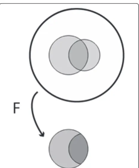
This situation is shown schematically in Figure 1 in which the area enclosed by the outer circle represents the entire patient population; the larger internal shaded region represents the number of patients with fever; the smaller internal shaded region represents the number of patients with appendicitis; and the area of overlap repre-sents the number of patients with both appendicitis and fever.
replacing the prior probabilityPr(A) with the true posi-tive ratePr(F|A), thus confusing the latter with the cor-rect quantity,Pr(A|F) [11,12,61]. The correct answer is computed by taking the fraction of patients with appen-dicitis among those with fever, Pr(A|F) = TP/(TP + FP) = 62/174 = 36%. Figure 1 illustrates this calculation graphically, where the act of taking fever as‘given’ is depicted as collapsing the population to just those patients who have fever. As expected, finding that a patient with abdominal pain has fever increases the probability of appendicitis - in fact, the probability more than triples (from 11% to 36%) - but, critically, the prob-ability increases from the prior probprob-ability Pr(A). One needs to know the prior probability Pr(A) to calculate the posterior probabilityPr(A|F).
Varying Pr(F|A)",1,0,2,0,0pc,0pc,0pc,0pc>>Varying Pr(F|A) Suppose we increase the true positive ratePr(F|A) from 56% to 71% (Figure 2). This increases the posterior probability of appendicitis from 36% to 41%. These increases correspond to an increase in the number of
appendicitis patients who have fever from 62 to 79, or graphically to a 15% expansion of the part of the fever region that is within the appendicitis region, with the result that a 5% larger fraction of the fever region con-tains appendicitis. Conversely, a decrease in the true positive rate Pr(F|A) from 56% to 40% decreases the posterior probability Pr(A|F) from 36% to 29%. These changes correspond numerically to a decrease in the number of patients with fever and appendicitis from 62 to 45.
Varying Pr F A( | )
Next let us slightly increase the false positive rate
Pr F A( | ) from 13% to 15% (Figure 3). This pushes the posterior probability Pr(A|F) down from 36% to 31%, and corresponds numerically to increasing the number of febrile patients without appendicitis from 112 to 136, or graphically to a 2% growth of the part of the fever region that is outside the appendicitis region, with the result that the fractional area of the fever region covered by appendicitis shrinks by 5%.
Conversely, a decrease in the false positive rate
Pr F A( | ) from 13% to 10% pushes the posterior prob-ability Pr(A|F) up from 36% to 41%. This corresponds numerically to decreasing the number of febrile patients without appendicitis from 112 to 88, or graphically to a
Table 2 Hypothetical statistics for fever and appendicitis
TP | FP Pr(F|A) | Pr(A)
FN | TN Pr F A( | ) | Pr(A|F)
62 | 112 56% | 11%
49 | 777 13% | 36%
79 | 112 71% | 11%
32 | 777 13% | 41%
45 | 112 40% | 11%
66 | 777 13% | 29%
62 | 136 56% | 11%
49 | 753 15% | 31%
62 | 88 56% | 11%
49 | 801 10% | 41%
139 | 192 56% | 45%
111 | 558 26% | 42%
22 | 121 56% | 4%
18 | 839 13% | 6%
shrinkage of the part of the fever region that is outside the appendicitis region by 3%, with the result that the fractional area of the fever region covered by appendici-tis expands by 5%.
Varying Pr(A)
Finally, consider increasing the prior probability of appen-dicitisPr(A) from 11% to 25% while holding the true and false positive rates fixed at Pr(F|A) = 56% and
Pr F A( | )=26%. This change raises the posterior prob-abilityPr(A|F) from 36% to 42%. In the corresponding Venn diagram shown in Figure 4 increasingP(A) corre-sponds to simply increasing the area ofA;Pr(F|A) is held fixed by increasing the area ofFwithinAproportionately, whereas keeping the same value for Pr F A( | ) requires a compensatory shrinkage of the shape forF. Likewise, decreasing the prior probability from 11% to 4% lowers the posterior probability from 36% to 16%, which in the accompanying Venn diagram requires shrinkingA, shrink-ing the part ofFwithinAproportionately to holdPr(F|A) fixed, and stretching the shape ofFoutside ofAto main-tain the fixed value of Pr F A( | ). The numbers for this example are shown in Table 2 and Figure 4.
Summary of the general rules
These examples illustrate the following general princi-ples (assuming a‘positive’test result):
•Increasing the true positive rate (sensitivity) pushes the posterior probability upward, whereas decreasing the true positive rate pushes the posterior probability downward.
• Increasing the false positive rate (1-specificity) pushes the posterior probability downward, whereas
decreasing the false positive rate pushes the poster-ior probability upward.
•Increasing the prior probability pushes the posterior probability upward, whereas decreasing the prior prob-ability pushes the posterior probprob-ability downward.
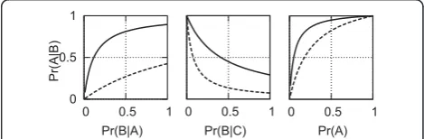
We emphasize again that in every case the posterior probability goes up or down from the prior probability, rather than being replaced by any of the three quantities. These general rules are illustrated in the graphs in Figure 5.
End of Part I
Uncertainty suffuses every aspect of the practice of medi-cine, hence any adequate model of medical reasoning, nor-mative or descriptive, must extend beyond deductive logic. As was believed for many decades, and recently proven by Cox and Jaynes, the proper extension of logic is in fact probability theory, with Bayes’rule as the central rule of inference. We have attempted to explain in an accessible way why Bayes’rule has its particular form, and how its behaves when its parameters vary. In the Part II, we inves-tigate ways in which probability theory is commonly mis-understood and abused in medical reasoning, especially in interpreting the results of medical research.
Discussion, Part II: significance testing
Every experiment may be said to exist only in order to give the facts a chance of disproving the null hypothesis. - RA Fisher [27]
Figure 2 Effects on posterior probability of changes in sensitivity, while holding prior probability and false positive rate constant.
Figure 3Effects on posterior probability of changes in false positive rate, while holding prior probability and sensitivity constant.
Figure 4Effects on posterior probability of changes in prior probability, while holding sensitivity and false positive rate constant.
0 0.5 1
0 0.5 1
Pr(A|B)
0 0.5 1 0 0.5 1
Pr(B|A) Pr(B|C) Pr(A)
Figure 5Illustration of how the posterior probability depends on the three parameters of Bayes’rule. Each plot shows two curves for the posterior probability as a function of one of the three parameters (with the remaining two parameters held constant) chosen from among one of two sets of values for(Pr(A),Pr(F|A),
Armed with our understanding of the anatomy and physiology of Bayes’rule, we are prepared for pathophy-siology. In Part II we explore common misinterpreta-tions and misuses of elementary medical statistics that occur in the application of significance testing, and how these can be effectively treated by applying our under-standing of Bayes’rule.
Before one can appreciate the problems with signifi-cance testing, one needs a clear understanding of a few concepts from ‘classical statistics’, namely binary hypothesis testing and P-values. We now proceed to review these concepts.
Binary hypothesis testing
Binary hypothesis testing is familiar to most physicians as the central concept involved in judging the results of clinical trials. The basic setup was encountered in the quiz that began the paper. For any propositionA, we set up two hypotheses:H0 =‘Ais not true’, called the null
hypothesis; and H1 =‘Ais true’, called the alternative
hypothesis. In our quiz, the effect of a new drug was being investigated and we had H0 = ‘the drug has no
effect’vs.H1 =‘the drug has some effect’. One of these
statements must be true as a matter of logical necessity. To find out which one, an experiment is carried out (for example a clinical trial), resulting in data D. We then conclude, through a procedure described below, that the data either favorsH0, called‘affirming the null
hypoth-esis,’or favorsH1, called‘rejecting the null hypothesis.’
We will denote our conclusions as eitherD0 =‘the data
favor the null hypothesis’, or D1 =‘the data favor the
alternative hypothesis’.
Our conclusions can be right or wrong in four ways (see Table 2). Correct results include ‘true positives’ (concluding D1 when H1 is true), and ‘true negatives’
(concluding D0 when H0 is true); the corresponding
probabilities Pr(D0|H0) and Pr(D1|H1) are called the
‘specificity’ and ‘power’ of the study, respectively. Incorrect results include Type I errors (concluding D1
when H0 is true), and Type II errors (concludingD0
when H1 is true); the corresponding probabilities Pr
(D1|H0) and Pr(D0|H1) are called the‘Type I error rate’
and‘Type II error rate’, respectively. There is a perfect analogy (and mathematically, no difference) between these probabilities and the ‘four fundamental forward probabilities’ well known to physicians in the context of diagnostic testing, namely, the true and false posi-tive rates, and true and false negaposi-tive rates. Similarly, corresponding to the‘four fundamental inverse prob-abilities’ of diagnostic testing, namely positive and negative predictive values and the false detection rate and false omission rate, there are exactly analogous quantities for the hypothesis testing scenario, that isPr (H0|D0),Pr(H1|D1), Pr(H0|D1), andPr(H1|D0). (See the
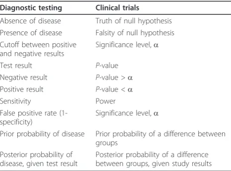
Additional file 1 for a brief review of the fundamental forward and backward probabilities of diagnostic test-ing.) This analogy is summarized in Table 3 and has been expounded beautifully in a classic paper by Browner and Newman [63]. We will return to this ana-logy near the end of the paper.
The null hypothesis significance testing procedure Let us now consider the conventional statistical reasoning process followed in drawing conclusions about experi-ments. This reasoning is prescribed by a standardized sta-tistical procedure, the‘null hypothesis significance testing procedure’(NHSTP), or simply‘significance testing’, con-sisting of the following steps.
1. Specify mutually exclusive and jointly exhaustive hypothesesH0 andH1.
2. Design an experiment to obtain dataD, and define a test statistic, that is a number or series of numbers that summarize the data,T=T (D) (for example the mean or variance).
3. Choose a minimum acceptable level of Type I error, called the‘significance level’, denoteda 4. Do the experiment, yielding dataD, and compute the test statistic,T =T(D).
5. Compute the P-value of the data from the test statistic, P=P(T(D)).
6. Compare the P-value to the chosen significance level. IfP≤a, conclude thatH1is true. IfP>a,
con-clude thatH0is true.
In the customary statistical jargon, whenP≤a, we say that the experimental results are‘statistically significant’, otherwise, they ‘do not reach significance.’ Also, note that the P-value itself is a statistic, that is a number computed from the data, so in effect we compute a test
Table 3 The analogy between diagnostic tests and clinical trials
Diagnostic testing Clinical trials
Absence of disease Truth of null hypothesis Presence of disease Falsity of null hypothesis Cutoff between positive
and negative results
Significance level,a
Test result P-value
Negative result P-value >a Positive result P-value <a
Sensitivity Power
False positive rate (1-specificity)
Significance level,a
Prior probability of disease Prior probability of a difference between groups
Posterior probability of disease, given test result
statistic T = T (D), from which we compute a second test statisticP = P(T(D)).
P-values
We now review whatP-values mean. The technical defi-nition that we will use differs in important ways infor-mal definitions more familiar to physicians, and the difference turns out to be consequential, as witnessed by the existence of a large critical literature dealing with practical and philosophical problems arising from defini-tions in common use [5,7,13-17,26,28,50,64-83]. As an overview to our own discussion of the conceptual issues at stake, we note that the literature critical ofP-values can be roughly divided into two dominant themes [75]. First, there are problems of interpretation. For example, consider the commonly encountered informal definition of theP-value as the probability that the observed result could have been produced by chance alone
The probability that the observed result could have been produced by chance alone
This definition is vague, and tempts many users into confusing the probability of the hypothesis given the data with the probability of the data given the hypothesis [13,17], that is it is unclear whether this definition refers to a conditional probability with the hypothesis H0 before the conditioning line,Pr(H0|·), or after the condi-tioning line,Pr(·|H0), which have very different meanings. Another common complaint is that the conventional cut-off value for‘significance’ofP< 0.05 is arbitrary. Finally, many have argued that real-world null hypotheses of‘no difference’are essentially never literally true, hence with enough data a null hypothesis can essentially always be rejected with an arbitrarily smallP-value, casting doubt on the intrinsic meaningfulness of any isolated statement that‘P <x’.Asecond entirely different class ofP-value criticisms concerns problems of construction [7,26,28,75,83]. This critique maintains thatP-values as commonly conceived are in fact conceptually incoherent and meaningless, rather than simply being subject to mis-interpretation. The charges revolve around a more expli-cit yet still mathematically informal type of definition of theP-value such as
the probability that the data (that is the value of the summary statistic for the data), or more extreme results, could have occurred if the intended experi-ment was replicated many, many times, assuming the null hypothesis is true.
The potential morass created by this definition can be illustrated by imagining that an experimenter submits a set of data, consisting, say, of 23 data samples, to a
statistical computer program, which automatically com-putes a P-value. According to the definition above, to produce theP-value, the computer must implicitly make several assumptions, often violated in actual practice, about the experimenter’s intentions, such as the assumption that there was no intention to: collect more or less data based on an analysis of the initial results (the‘optional stopping problem’); replace any lost data by collecting additional data; run various conditions again; or compare the data with other data collected under different conditions [26,28,75]. Any of these alter-native intentions would leave the actual data in hand unaltered, while implicitly altering the null hypothesis, either trivially by changing the number of data points that would be collected in repeated experiments, or by more profound alterations of the precise mathematical form of the probability distribution describing the null hypothesis. Consequently, theP-value apparently varies with the unstated intentions of the experimentalist, which in turns means that, short of making unjustified assumptions about those intentions, theP-value is math-ematically ill defined.
In what follows, we will avoid the ‘constructional’ objections raised above by using a mathematically expli-cit definition for the P-value. Problems with interpreta-tion will still remain, and the following secinterpreta-tion will focus in detail on what we believe are the most serious of the common modes of misinterpretingP-values. The generally accepted mathematical definition for the P-value is [84]:
the probability under the null hypothesis of obtain-ing the same or even less likely data than that which is actually observed, that is the probability of obtain-ing values of the test statistic that are equal to or more extreme than the value of the statistic actually computed from the data, assuming that the null hypothesis is true.
a mathematically complicated form. Methods for specify-ing and computspecify-ing complex null hypotheses are beyond the scope of this essay, but have been well worked out in a wide variety of practically important cases, and are in wide use in the field of statistics. The important point to grasp here is that once the null hypothesisH0, is specified, or more precisely, the relevant probability distributionPr(T (D)|H0), then computing theP-value can in principle pro-ceed in a straightforward, uncontroversial manner, accord-ing to its mathematical definition given above. As mentioned above, without specifying the null hypothesis distribution explicitly, theP-value is ill-defined, because any raw data are generally consistent with multiple differ-ent possible sample-generation processes, each which of may entail a differentP-value [25,26].
We now turn to explaining our final, technical defini-tion of the P-value. We will do this by exploring the definition from the vantage point of three different examples. The third example presents an additional, alternative definition ofP-values which provides novel insights into the true meaning ofP-values by viewing them from the medically familiar perspective of sensitiv-ity and specificsensitiv-ity considerations, in the context of ROC curves. This final definition will be mathematically equivalent, though not in an immediately obvious way, to the definition just given.
Angle 1. P-values as tail area(s)
Graphically, aP-value can be depicted as the area under one or two tails of the null-hypothesis probability distri-bution for the test statistic, depending on the details of the hypothesis being tested. For example, consider the classification of patients’systolic blood pressure as either chronically hypertensive, H1, or not chronically
hyper-tensive,H0, on the basis of a single blood pressure
mea-surement. Let us assume that blood pressures for normotensive patients obey a normal distribution (BP), as shown in Figure 6. If for a particular patient we obtain a systolic blood pressure of SBP= 138.6, then the P-value for this result is the probability in a non-hypertensive patient of finding a blood pressure equal to or greater than this value, or the area under the right sided tail of (BP), starting fromSBP=138.6.
If instead the null hypothesis states that the patient is chronically normotensive,H0, so that the alternativeH1
includes the possibility of either hypertension or hypo-tension, then the P-value would be ‘two-sided’, since values under an equally-sized left sided tail of the distri-bution would be equally contrary to the hypothesisH0
and hence would have caused us to reject H0according
to the null hypothesis significance testing procedure (NHSTP).
Angle 2. P-values for coin flipping experiments
Let us carry out the P-value calculation in detail for a simple coin flipping experiment, where we wish to
decide whether a coin is fair (equal probability of heads or tails) or biased (unequal probabilities). Note that the P-value in this case is‘two-sided’. Following the NHSTP:
1. Let H0 =‘the probability of heads is 1/2’, H1 =
‘probability of heads≠1/2’.
2. The experiment will consist of flipping a coin a number of timesn, and the dataD will thus be a series of heads or tails. For our test statisticT, let us compute the difference between 1/2 and the frac-tion of heads, that is ifkof the ncoin tosses land as heads, thenT(D) = |1/2-k/n|. For this example, let us putn= 10.
3. We set the significance level to the conventional valuea= 0.05 = 5%.
4. Having done the experiment suppose we get data D =(H, H, H, H, H, H, T, H, H, T). This sequence contains eight heads, soT(D) =|1/2-8/10| = 0.3. 5. To calculate theP-value, we must consider all the ways in which the data could have been as extreme or more extreme than observed, assuming that the null hypothesis is true. That is, we need to consider all possible outcomes for the dataDsuch thatT(D)
≥ 0.3, and calculate the joint probability of these outcomes, assuming that the coin is fair. Clearly, observing eight, nine, or ten heads would be ‘as extreme or more extreme’than our result of eight heads. Since the null hypothesis assumes equal prob-ability for heads and tails, symmetry dictates that observing zero, one, or two heads would also qualify. Hence, theP-value is:
p Pr T D H
Pr k k H
= ≥
= ≥ ≤
=
( ( ) . | )
( | )
. %. 0 2
8 2
10 94
0
0 or
(See Additional file 1 for details of this and the next two calculations.)
6. Sincep≥ 5%, the NHSTP tells us to accept the null hypothesis, concluding that the coin is fair.
0 0.01 0.02 0.03 0.04
80 90 100 110 120 130 140 150 160 SBP (mmHg)
Before leaving this example, it is instructive to exam-ine its associated Type I and II error rates. The Type I error rate (false positive rate) in this case is the prob-ability of incorrectly declaring the coin unfair (H1) when
in fact it is fair (H0), that is, the probability of getting P
≤ a when in fact H0 is true. It turns out that had we
observed just one more head then the NHSTP would have declared a positive result. That is, suppose k= 9, orT(D) = |1/2 - 9/10| = 0.4.
Then:
p Pr T D H
Pr k k H
= ≥
= ≥ ≤
=
( ( ) . | )
( | )
. %. 0 4
9 1
2 15
0
0 or
Thus, we see thatP ≤a wheneverd≥0.4, hence the Type I error rate or false positive rate is:
FPR=Pr D( 1|H0)=Pr p( ≤|H0)=2 15. %.
Calculation of the false negative rate requires addi-tional assumptions, because a coin can be biased in many (in fact, infinitely many) ways. Perhaps the least committed alternative hypothesis H1 is that for biased
coins any heads probability different from 1/2 is equally likely. In this case the false negative rate turns out to be FNR=Pr(D0|H1) = 72.73%
Angle 3: P-values from ROC curves
To take a third angle, we consider an alternative defini-tion for theP-value [84]. TheP-value is
the minimum false positive rate (Type I error rate) at which the NHSTP will reject the null hypothesis.
Though not obvious at first glance, this definition is mathematically equivalent to our previous definition of the P-value as the probability of a result at least as extreme as the one we observe. The effort required to see why this is the case affords additional insight into the nature ofP-values.
Let us step back and consider the null hypothesis test-ing procedure from an abstract point of view. The NHSTP is one instance of threshold-decision procedure, that is, a procedure that chooses between two alterna-tives by comparing a test statistic computed from the dataT(D) with a thresholdg(in the case of the NHSTP, the statistic is theP-value, and the threshold is the sig-nificance level a). The procedure declares one result when the test statistic is less than or equal to threshold, and the alternative result when the threshold is exceeded. Identifying one of the alternatives as ‘positive’ and the other as ‘negative’, in general any such thresh-old-based decision procedure must have a certain false positive and false negative rate, determined by the
chosen threshold. More explicitly, let us denote the positive and negative alternatives asH1 andH0,
respec-tively, and declare a positive result whenever T(D)≤g, or a negative result whenever T(D) >g. A false positive then occurs if T(D)≤ gwhen in factH0is true, and the
probability of this event is denoted FPR(g) =Pr(T(D)≤ g|H0). Similarly, a true positive result occurs ifT(D)≤g
when H1 is true, and the probability of this event is
denoted TPR(g) = Pr(T(D) ≤ g|H1). If we allow the
threshold to vary, we can generate a curve of the false positive rate versus the false negative rate; such a curve is called a ROC curve. To make this discussion concrete, let us return to our coin flipping example. In that case, we set the ‘positive’ alternative to H1 = ‘the coin is
biased’(that isPr(Heads|H1)≠1/2), and set the negative
alternative to H0 = ‘the coin is fair’ (Pr(Heads|H0) =
1/2). Setting the test statistic as before to T(D) = d= |1/2 -k/n|, we then have:
FPR Pr d H
TPR Pr d H
( ) ( | ),
( ) ( | ).
= ≥
= ≥
0
1
The resulting ROC curveROC(g) = (FPR(g),TPR(g)) is plotted in Figure 7. (On a technical note, the way we have set up our decision procedure, there are really only seven achievable values of (TPR(g),FPR(g)) on this ROC curve, marked by the circles: The first five values corre-spond to the five possible values of d, 0, 0.1, 0.2, 0.3, 0.4, which correspond in turn to the following pairs of possible values k for the number of heads in ten coin tosses (0. 10), (1. 9), (2. 8), (3. 7), (4. 6) (each member of the pair gives the same value for d); the sixth value corresponds to the valued= 0.5, which corresponds to a result of five heads; and the seventh value corresponds to setting the threshold to any value beyond what is
a b c d e
a b c d e
F
T
x
g h
i
j
k
l
m
obtainable, that is tog < 0. We have connected these seven points with straight lines to create a more aesthe-tically pleasing plot.)
Key points on the ROC curve are marked by circles, and the corresponding value for isgnoted. Points on the ROC curve‘down and to the left’(low false positive rate, low true positive rate) correspond to setting the thresh-old low; whereas values‘up and to the right’(high false positive rate, high true positive rate) correspond to set-ting the threshold high. Clearly, if we wished to avoid all false positive conclusions, we could set the threshold to -∞, since all results will then be declared negative (Pr(d≤ -∞|H0) = 0), but this comes at the expense of rejecting all
true positive results as well (sincePr(d≤-∞|H1) = 0).
Conversely, we can avoid missing any true positive results by setting the threshold tog≤0.5, since it is true for all possible results thatd≤0.5 (hencePr(d≤0.5|H1)
= 1), but this simultaneously results in a maximal false positive rate (sincePr(d≤0.5|H0) = 1 also). Clearly,
posi-tive results are only meaningful when obtained with the thresholdgset to some value intermediate between these extremes. Now, suppose that after conducting our coin flipping experiment we decide to‘cheat’as follows. As before let the outcome be that we get eight heads, ord= |1/2 - 8/10| = 0.3. Rather than choosing the decision threshold beforehand, we instead choose the threshold after seeing this result, to ensure that the result is declared positive. Our results will look best if we choose the thresholdgas small as we can, to let through as few false positives as possible, while still letting our result pass. This special choice of the thresholdgis clearly the value of our actual result, so we setg=d= 0.3, and voilà, our result is positive. We cannot make the false positive rate any smaller without making our result negative according to the NHSTP.
Now for the point of this whole exercise: If we drop a vertical line from the point on the ROC curveROC(0.3) = (TPR(0.3),FPR(0.3)) down to the x-axis to see where it intersects, we see that the false positive rate isFPR (0.3) = 10.94%, which is the result we calculated pre-viously as theP-value. Thus the condition for declaring a positive result (d≤ g) is equivalent to the condition in the NHSTP (P ≤ a), hence, as claimed, the P-value is the minimum false positive rate at which the NHSTP will reject the null hypothesis. As an immediate corol-lary we also see that false positive rate of the NHSTP is simply the significance level, that is:
Pr D( 1|H0)=Pr P( ≤|H1)=
Is significance testing rational?
The null hypothesis significance test (NHST) should not even exist, much less thrive as the dominant
method for presenting statistical evidence. . . It is intellectually bankrupt and deeply flawed on logical and practical grounds. - Jeff Gill [85]
We are now in a position to answer the question: Is the null hypothesis significance testing procedure a rational method of inference? We will show momenta-rily that the answer is a resounding ‘NO!’, but first we briefly consider why, despite its faults, many find it intuitively plausible. Several books explore the reasons in detail [59,86-88], and a full account is well beyond the scope of this paper. We will focus on one particu-larly instructive explanation, called‘the illusion of prob-abilistic proof by contradiction’ [13]. Consider once again the valid logical argument form:
if is true, then is true. is false.
is false.
A B
B A
∴
This argument is called ‘proof by contradiction’: Ais proved by ‘contradicting’B, that is the falsehood of A follows from the fact thatB is false. It is tempting to adapt this argument for use in uncertain circumstances, like so:
If is true, then is probably true is false
is false.
A B
B A
. .
∴
By analogy, this argument could be called‘ probabilis-tic proof by contradiction’. However, this analogy quickly dissolves after a little reflection: The premise (that is the‘if, then’statement) leaves open the possibi-lity that A may be true while B is nonetheless false. More concretely, consider the statement ‘If a woman does not have breast cancer, then her mammogram will probably be negative.’(This example is discussed more extensively in an excellent online tutorial by Eliezer Yudkowsky [61].) This statement is true. However, given a positive mammogram, one cannot invariably pro-nounce a diagnosis of breast cancer, because false posi-tives do sometimes occur. This simple example makes plain that‘probabilistic proof by contradiction’is an illu-sion - it is not a valid argument. And yet, this is literally the form of argument made by the NHSTP. To see this, simply make the following substitutions:
A=‘H0is true’, andB=‘P>a’, to get:
If is true, then probably
is false
H P
p H
0
0
> ≤
∴
. .
Again, we have just seen that this is an invalid argu-ment. One obvious‘fix’is to try softening the argument by making the conclusion probabilistic:
If is true, then probably
is probably false
H P
P H
0
0
> ≤
∴
. .
.
Unfortunately, any apparent validity this has is still an illusion. To see the problem with this argument, let us return to the mammography example. Is it rational to conclude that a positive mammogram implies that a woman probably has breast cancer? The correct answer, obvious to most physicians at an intuitive if not at a for-mal statistical level is, ‘it depends on the patient’s clini-cal characteristics, and on the quality of the test’. Very well, then let us give a bit more information: Suppose that mammography has a false positive rate of 20%, and sensitivity of 80%. Can we now assign a probable diag-nosis of breast cancer? Interestingly, most physicians answer this question affirmatively, giving a probability of cancer of 80%, a conclusion apparently reached by erro-neously replacing the sensitivityPr(H1|D1) with the
posi-tive predicposi-tive valuePr(D1|H1) [9,11,12]. The fallacy here
has been satirized thus:
It is like the experiment in which you ask a second-grader: ‘If eighteen people get on a bus, and then seven more people get on the bus, how old is the bus driver?’ Many second-graders will respond: ‘Twenty-five.’....Similarly, to find the probability that a woman with a positive mammography has breast cancer, it makes no sense whatsoever to replace the original probability that the woman has cancer with the probability that a woman with breast cancer gets a positive mammography. - Eliezer Yudkowsky [61]
To calculate the desired probability Pr(H1|D1)
cor-rectly, Bayes’rule requires that we also know the prior probability of disease. Suppose that our patient is a healthy young woman, from a population in which the prevalence of breast cancer is 1%. Then, given her posi-tive mammogram the probability that she has breast cancer is:
Pr H D( ) (. )(. )
(. )(. ) (. )(. ) . %.
1 1
80 01
8 1 99 2 7 8
=
+ =
To put it as alarmingly as possible, the probability that she has breast cancer has increased by almost 8 fold! Nevertheless, she probably does not have cancer (7.8% is far short of 50%); the odds are better than nine to one against it, despite the positive mammogram. Thus, while further testing may be in order, a rational response is
reassurance and perhaps further investigation rather than pronouncement of a cancer diagnosis. This and other examples familiar from everyday clinical experi-ence make clear that the null hypothesis significance testing procedure cannot‘substitute’for Bayes’rule as a method of rational inference.
We have focused our criticism on what we consider to be the most fundamental and most common error in the interpretation of P-values, namely, the error of mis-taking‘significant’P-values as proof that a hypothesis is ‘probably true’. There are many other well documented conceptual problems with P-values as commonly employed which we have not discussed. The interested reader is referred to the excellent discussions in the fol-lowing references [7,28].
Answers to the quiz
The answer to the quiz at the beginning of this paper is plain from the preceding discussion. Given a P-value that reaches significance (such that the NHSTP would have us conclude thatH1 is true), what conclusions are
we actually justified in drawing regarding the probability that either hypothesisH1 orH0is true? Answers (1), (2),
and (5) are incorrect because the NHSTP, which corre-sponds to the ‘hard’version of ‘probabilistic proof by contradiction’is an invalid argument. Answers (3), (4), and (6) are invalid because the‘softened’version of the same argument is still invalid.
To determine the probability that H1 is actually true
in light of the positive result D1 =‘P<a’, that is, to
cal-culate Pr(H1|D1), Bayes’rule requires that we have three
pieces of information. First, we need the false positive rate, which as we have seen for the NHSTP isPr(D1|H0)
=Pr(P≤a|H0) =a; this is the only piece of information
we were given in the quiz question. Second and third, however, we need to know the ‘power’(sensitivity) of the study, Pr(D1|H1), and the pre-test probability of the
hypothesis, Pr(H1). Thus, the correct answer is ‘(7)
None of the above’.
Do prior probabilities exist in science?
Though most physicians are comfortable with the con-cept of prior probability in the context of diagnostic test interpretation, many are less comfortable thinking about prior probabilities in the context of interpreting medical research data. As one respondent to our quiz thought-fully objected,
convince us that the pre-test probability is reasonably high so that a result will be accepted. They do this by laying the scientific groundwork (introduction), laying out careful methods, particularly avoiding bias and confounders (methods), and describing the results carefully. Thereafter, they use the discussion section to outright and unabashedly try to convince us their results are right. But in the end, we do the positive predictive value calculation in our head as we read a paper... As an example, one person reads the SPARCL study and says, ‘I do not CARE that the P-value shows statistical significance, it is hooey to say that statins cause intracranial hemorrhage.’... They have set a very low pre-test probability in their head. Another person reads the same study and says, ‘I have wondered about this because I have seen lots of bleeds in people on statins.’They have set a much higher pre-test probability.
This response actually makes our point, perhaps inad-vertently, about the necessity of prior probabilities. Nevertheless, several important points raised by this response warrant comment.
Do prior probabilities‘exist’in science?
First, to the philosophical question of whether prior probabilities‘exist’in science, the answer is‘yes and no’. On the one hand, probability theory is always used as a simplifying model rather than a literal description of reality, whether in science or clinical testing (with the possible exception of probabilities in quantum mechanics). Thus, when one speaks of the probability that a coin flip will result in heads, that a drug will have the intended effect, or that a scientific theory is correct, one is not necessarily committing to the view that nat-ure is truly random. In these cases, the underlying rea-lity may be deterministic (for example a theory is either true or false), in which referring to probabilities repre-sents merely a convenient simplification, but do not really ‘exist’in the sense that they would not be needed in a detailed, fundamental description of reality. How-ever, simplification is essentially always necessary in dealing with any sufficiently complex phenomena. For example, while it might be possible to conceive of a supercomputer capable of predicting the effects of a drug using detailed modeling of the molecular interac-tions between the drug and the astronomical number of cells and molecules in an individual patient’s body, in practice we must make predictions with much less com-plete information, hence we use probabilities. The use of such simplifications is no less important in scientific thinking than in medical diagnostic testing. Thus, inso-far as probabilities ‘exist’ at all, they are not limited to the arena of diagnostic testing.
Are prior probabilities in science arbitrary?
Given that prior probabilities for hypotheses in science and medicine are often difficult to specify explicitly in precise numerical terms, does this mean that any prior probability for a hypothesis is as good as any other? There are at least two reasons that this is not the case. First, pragmatically, people do not treat prior probabil-ities regarding scientific or medical hypotheses as arbi-trary. To the contrary, they go to great lengths to bring their probabilities into line with existing evidence, usually by integrating multiple information sources, including direct empirical experience, relevant theory (for example an understanding of physiology), and lit-erature concerning prior work on the hypothesis or related hypotheses. These prior probability assignments help scientists and physicians choose which hypotheses deserve further investment of time and resources. More-over, while these probability estimates are individualized, this does not imply that each person’s‘subjective’ esti-mate is equally valid. Generally, experts with greater knowledge and judgement can be expected to arrive at more intelligent prior probability assignments, that is their assignments can be expected to more closely approximate the probability an ‘ideal observer’ would arrive at based on optimally processing all of the exist-ing evidence. Second, in a more technical vein, methods for estimating accurate prior probabilities from existing data are an active topic of research, and are likely to lead to increased and more explicit use of‘Bayesian sta-tistics’in the medical literature [29,31-36,83,89].
Taking responsibility for prior probabilities
Has significance testing been perverted?
Considering the criticisms we have reviewed, it is nat-ural to ask whether significance testing is being used as its originators intended. Significance testing is actually an amalgam of two approaches to statistical inference, developed on the one hand by RA Fisher, who invented the concept of P-values, and on the other hand by J Neyman and K Pearson, who together developed the theory of binary hypothesis testing. Hypothesis testing and P-values were combined into the method of null hypothesis significance testing by others, to the chagrin of Fisher, Neyman and Pearson, who were vigorously outspoken critics of one another’s methods [16,17]. In this connection, the following quotation from Neyman and Pearson on their philosophy towards hypothesis testing (of which significance testing is a special case) is particularly interesting:
...no test based upon a theory of probability can by itself provide any valuable evidence of the truth or falsehood of a hypothesis. . . But we may look at the purpose of tests from another viewpoint. Without hoping to know whether each separate hypothesis is true or false, we may search for rules to govern our behavior with regard to them, in following which we insure that, in the long run of experience, we shall not often be wrong [101].
Thus, Neyman and Pearson apparently did not intend hypothesis testing to be used as it usually is used nowa-days, as a method for appraising the truth of individual hypotheses. Rather, their method was intended merely to be correct in an aggregate sense. While this may be
acceptable, say, to decide the fates of mass-produced objects in an industrial setting, it is unsatisfactory in medical situations involving individuals. There, it is imperative that we strive to be right in each case. Simi-larly, few researchers would be content to use a method of inference realizing that it cannot accurately appraise the truth of the individual hypotheses. While signifi-cance testing does not provide a way to know‘whether each separate hypothesis is true or false’, fortunately Bayes’rule does provide rational grounds for appraising the strength of evidence in favor of individual hypotheses.
How significant is a significant result?
If it is unjustified to regard a ‘statistically significant’ result as sufficient evidence for the truth of a hypothesis, then what can we conclude when we read‘P≤ a’? How much evidence does a statistically significant result pro-vide for its hypothesis? The fact is that the amount of evidence provided by a P-value depends on the prior probability and power of the research methodology, in the way prescribed by Bayes’rule. Thus, there is no gen-eric value of Pthat will render a hypothesis more likely true than not (that is Pr(H1|P≤ a) > 50%). Rather, the
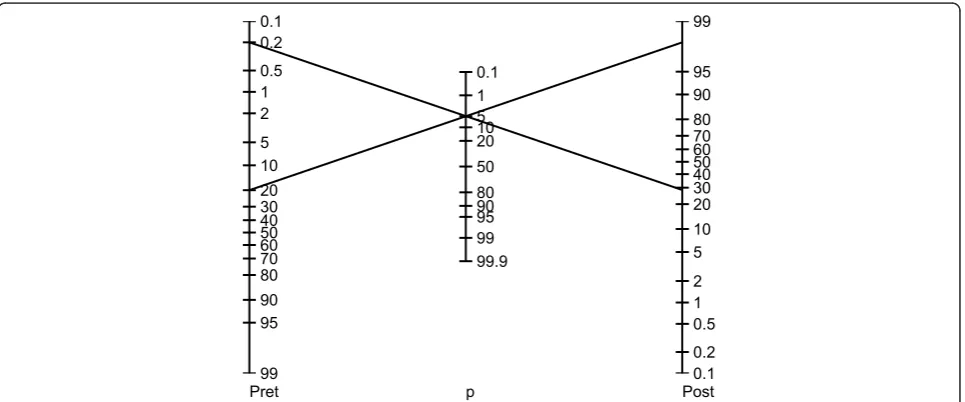
true‘significance’ of Pvaries from case to case, in the same way as the meaning of a BNP value varies accord-ing to a patient’s clinical characteristics when evaluating for suspected congestive heart failure (see Additional file 1 Figure S1) [102,103]. It is helpful conceptually when assessingP-values to envision a’P-value nomogram’, as illustrated in Figure 8. As shown, aP-value of 0.05 can lead to very different posterior probabilities. Note that the particular nomogram shown is not universal; it was
0.1 0.2 0.5 1 2
5 10 20 30 40 50 60 70 80 90 95
99 0.1
0.2 0.5 1 2 5 10 20 30 40 50 60 70 80 90 95 99
0.1 1 5 10 20 50 80 90 95 99 99.9
Pret p Post
calculated by assuming specific distributions for H0 and
H1. But the basic idea that the degree of support for a
hypothesis provided by a P-value depends on the pre-test probability is general.
Are physicians good Bayesians?
Probability theory was regarded by its early architects as a model not only for how educated minds should work, but for how they do actually work. This ‘probabilistic theory of mind’ forms the basis for modern views on the nature of rationality in philosophy, economics, and more recently in neuroscience [104-108]. How can this be, when there is widespread misunderstanding of the most basic of statistical concepts likeP-values and sig-nificance testing, even among a group as educated and accustomed to consuming statistical data as physicians? We briefly consider arguments for and against the possi-bility that physicians are, or can be, good Bayesians.
Anti-Bayes
In his evaluation of the evidence, man is apparently not a conservative Bayesian: he is not a Bayesian at all. - Kahneman and Tversky [109]
The most serious challenge to the probabilistic theory of mind is the ‘heuristics and biases’ movement of experimental psychology, started by a series of influen-tial papers published in the late 1960 s and early 1970 s by Kahneman and Tversky [109,110]. The central claim of this movement is that people tend to make judge-ments under uncertainty not according to Bayes’rule, but instead by simplifying rules of thumb (heuristics) that, while convenient, nevertheless often lead to sys-tematic errors (biases). With respect to medical reason-ing, we can roughly categorize the types of biases by whether they affect one’s clinical estimates of prior or posterior probabilities.
Prior (pre-test) probabilities
Physicians’ estimates of the prior probability of disease may vary wildly [10,111,112]. For example, given the same vignette of the history, physical exam, and EKG for 58 year old female with chest pain, physicians were asked to assign probabilities to various diagnoses includ-ing acute myocardial infarction (AMI), aortic dissection, and gastroesophageal reflux. Estimates for AMI ranged from 1% to 99%, and the probabilities assigned by many physicians surveyed added to greater than 100% [10]. Two classic examples of cognitive biases that contribute to this variability are the representativeness and avail-ability biases.
Representativeness biasThis is the tendency to violate the old medical maxim,‘when you hear hoofbeats, think horses, not zebras.’That is, the tendency to set the prior probability inappropriately high for rare diseases whose
typical clinical presentation matches the case at hand, and inappropriately low for common diseases for which the presentation is atypical. This bias leads to overdiag-nosis of rare diseases.
Availability bias Also called the ‘last case bias’in the medical context, this is the tendency to overestimate the probability of diagnoses that easily come to mind, as when, having recently seen a case of Hashimoto’s ence-phalopathy, one automatically suspects this first in the next patient who presents with confusion, a relatively nonspecific sign. Another example is doubting that smoking is harmful because one’s grandmother was a smoker yet lived to age ninety.
Posterior (post-test) probabilities
Other studies have explored ways in which physicians deviate from Bayes’ rule in updating prior probabilities in light of new data [113,114]. Well known examples of responsible underlying cognitive biases are the anchor-ing, confirmation, and premature closure biases.
Anchoring biasThis is the tendency to set one’s poster-ior probability estimate inappropriately close to a start-ing value, called an anchor. Errors can arise from anchoring to an irrelevant piece of information (as when patients are sent home from the low-acuity part of the emergency department who would have been admitted from the high-acuity part), or by generally undervaluing new information when it does not support one’s initial impression.
Confirmation biasAlso known as belief preservation, hypothesis locking, and selective thinking, this is the tendency maintain one’s favored hypothesis by overvalu-ing and selectively searchovervalu-ing for confirmatory evidence and undervaluing or ignoring contradictory evidence. Reasons for this bias include vested emotional interest, for example as when avoiding a potentially upsetting diagnosis, or inconvenience, for example as when down-playing medical symptoms in a patient with challenging psychiatric problems.
Premature closure biasThis is the tendency to make a diagnosis before sufficient evidence is available. Prema-ture closure bias can arise from emotional factors such as discomfort over a patient’s or the physician’s own uncertainty, or because of time pressure [113,114].
Pro-Bayes
[T]he theory of probability is at bottom nothing more than good sense reduced to a calculus which evaluates that which good minds know by a sort of instinct, without being able to explain how with pre-cision. - Laplace [115]
![Figure 6 Distribution of systolic blood pressures for apopulation of healthy 60-69 year old males (from data in[125])](https://thumb-us.123doks.com/thumbv2/123dok_us/8911624.1836939/10.595.306.537.89.191/figure-distribution-systolic-blood-pressures-apopulation-healthy-males.webp)