Issues
ISSN: 2146-4138
available at http: www.econjournals.com
International Journal of Economics and Financial Issues, 2018, 8(2), 304-314.
Import Components and Import Multipliers in Australian
Economy: Wor
l
d Input - Output Analysis
M. Muchdie
1*, H. Kurniawan
21Department of Management, Graduate School, Universitas Muhammadiyah Prof. Dr. HAMKA, Jakarta, Indonesia, 2Department
of Management, Faculty of Economics and Business, Universitas Muhammadiyah Prof. Dr. HAMKA, Jakarta, Indonesia. *Email: [email protected]
ABSTRACT
This article analysis on import components and import multipliers, using Australian input-output tables 2000, 2005, 2010 and 2014. The results
showed that firstly, Australian import components of input were, on average, <20%; meaning that input that locally provided were more than 80%. Australian import of input had increased significantly from US$ 47,122 million in 2000 to US$ 14,616 million in 2014. Secondly, Australian imports have been dominated by Sector-8, Sector-13, Sector-24, Sector-25, and Sector-26. Thirdly, Australian imports have been dominated by the USA, Japan, United Kingdom, China and Germany. During 2000-2014, import from Canada, Japan, UK and the USA had declined, but import from China had significantly increased. Finally, highest sectoral import multipliers occurred in Sector-5, Sector-22, Sector-29, Sector-30, Sector-31, and Sector-32, but there was no significant different of import multipliers for country origin of import.
Keywords: Import Components, Sectoral Import Multipliers, Spatial Import Multipliers
JEL Classifications: C67, D57, F17
1. INTRODUCTION
Imports consist of transactions in goods and services to a resident of a jurisdiction such as a nation from non-residents (Lequiller
and Blades, 2006). An import of a good occurs when there is a
change of ownership from a non-resident to a resident. Imports of services consist of all services rendered by non-residents to residents. In national accounts, import includes and excludes
specific “borderline” cases. In macroeconomic theory, the value of
imports can be modelled as a function of the domestic absorption
and the real exchange rate Burda (2005). There are two basic types
of import: Industrial and consumer goods and intermediate goods and services. Companies import goods and services to supply to the domestic market at a cheaper price and better quality than competing goods manufactured in the domestic market.
Australian intermediate input that imported has increase
significantly during 2000-2014 (Muchdie, 2017). Trinh et al. (2008) explained that imported intermediate input was shown
in the usual Keynesian foreign trade multiplier analysis. In an
open economy, Y+M = C+I+E; the external sector is combined inconsistently with the domestic sector in the circular flow. Where, Y stands for net national products (or net final demand)
excluding intermediate products, while M stands for imported including intermediate products. On the other hand, Leontief’s matrix multiplier is devoted entirely to the analysis of intermediate
products in the circular flow, the Leontief system can regard the
household sector as an industry whose output is labor income and
inputs are consumption products; an analysis of the multiplier
process via the consumption function.
The objective of this paper is to analyse import components and
the impact of final demand change on Australian imports, known as import multipliers, using Australian 37 sector input-output tables of
years: 2000, 2005, 2010 and 2014 from World Input-Output Tables.
2. LITERATURE REVIEW
good is called an importer (Joshi, 2009). An import in the receiving
country is an export from the sending country. Importation and
exportation are the defining financial transactions of international
trade. In international trade, the importation and exportation of goods are limited by import quotas and mandates from the customs authority. Imports consist of transactions in goods and services to a resident of a jurisdiction such as a nation from non-residents
(Lequiller and Blades, 2006). An import of a good occurs when
there is a change of ownership from a non-resident to a resident. Imports of services consist of all services rendered by non-residents to residents. In national accounts, import includes and excludes
specific “borderline” cases. In macroeconomic theory, the value of
imports can be modelled as a function of the domestic absorption
and the real exchange rate (Burda, 2005). There are two basic types
of import: Industrial and consumer goods and intermediate goods and services. Companies import goods and services to supply to the domestic market at a cheaper price and better quality than competing goods manufactured in the domestic market. Trinh et al.
(2008) explained that imported intermediate input was shown in
the usual Keynesian foreign trade multiplier analysis.
In macroeconomics, a multiplier is a factor of proportionality that measures how much an endogenous variable changes in response to a change in some exogenous variable (see among others:
Dornbusch and Stanley, 1994; McConnell et al., 2011; Pindyck and Rubinfeld, 2012). In monetary microeconomics and banking, the
money multiplier measures how much the money supply increases in response to a change in the monetary base (see among others:
Krugman and Wells, 2009; Mankiw, 2008). Multipliers can be calculated to analyze the effects of fiscal policy, or other exogenous changes in spending, on aggregate output. Other types of fiscal
multipliers can also be calculated, like multipliers that describe the effects of changing taxes.
Literature on the calculation of Keynesian multipliers traces back to Kahn’s description of an employment multiplier for government
expenditure during a period of high unemployment (Kahn, 1931).
At this early stage, Kahn’s calculations recognize the importance of supply constraints and possible increases in the general price level resulting from additional spending in the national
economy (Ahiakpor, 2000). Hall (2009) discusses the way that
behavioural assumptions about employment and spending affect econometrically estimated Keynesian multipliers.
The literature on the calculation of I-O multipliers traces back to
Leontief (1951), who developed a set of national-level multipliers
that could be used to estimate the economy-wide effect that an
initial change in final demand has on an economy. Isard (1951) then
applied input-output analysis to a regional economy. According to
Richardson (1985), the first attempt to create regional multipliers
by adjusting national data with regional data was Moore and
Peterson (1955) for the state of Utah. In a parallel development, Tiebout (1956) specified a model of regional economic growth
that focuses on regional exports. His economic base multipliers are based on a model that separates production sold to consumers from outside the region to production sold to consumers in the region. The magnitude of his multiplier is based on the regional supply chain and local consumer spending.
In a survey of input-output and economic base multipliers,
Richardson (1985) notes the difficulty inherent in specifying
the local share of spending. He notes the growth of
survey-based regional input-output models in the 1960s and 1970s that
allowed for more accurate estimation of local spending, though at a large cost in terms of resources. To bridge the gap between
resource intensive survey-based multipliers and “off-the-shelf” multipliers, Beemiller (1990) of the BEA describes the use of
primary data to improve the accuracy of regional multipliers. The literature on the use and misuse of regional multipliers and
models is extensive. Coughlin and Mandelbaum (1991) provide an
accessible introduction to regional I-O multipliers. They note that key limitations of regional I-O multipliers include the accuracy of leakage measures, the emphasis on short-term effects, the absence of supply constraints, and the inability to fully capture interregional feedback effects.
Grady and Muller (1988) argued that regional I-O models that
include household spending should not be used and argue that
cost-benefit analysis is the most appropriate tool for analyzing the benefits of particular programs. Mills (1993) noted the lack
of budget constraints for governments and no role for government debt in regional IO models. As a result, in less than careful hands, regional I-O models can be interpreted to over-estimate
the economic benefit of government spending projects. Hughes (2003) discussed the limitations of the application of multipliers
and provides a checklist to consider when conducting regional
impact studies. Harris (1997) discussed the application of regional
multipliers in the context of tourism impact studies, one area where
the multipliers are commonly misused. Siegfried et al. (2006)
discussed the application of regional multipliers in the context of college and university impact studies, another area where the multipliers are commonly misused. Input-output analysis, also known as the inter-industry analysis, is the name given to an
analytical work conducted by Leontief in the late 1930’s. The
fundamental purpose of the input-output framework is to analyze the interdependence of industries in an economy through market-based transactions. Input-output analysis can provide important and timely information on the interrelationships in a regional economy and the impacts of changes on that economy.
The notion of multipliers rests upon the difference between the
initial effect of an exogenous change (final demand) and the total
effects of a change. Direct effects measure the response for a given
industry given a change in final demand for that same industry.
Indirect effects represent the response by all local industries from
a change in final demand for a specific industry. Induced effects
represent the response by all local industries caused by increased
(decreased) expenditures of new household income and inter-institutional transfers generated (lost) from the direct and indirect effects of the change in final demand for a specific industry. Total
effects are the sum of direct, indirect, and induced effects.
In input-output model, multipliers were distinguished by output,
income, employment and other value added. West (1990) defined
total output multipliers as summation of initial, direct, indirect
output multiply by direct requirement of household coefficients of income. Import multipliers can be defined as impact of direct, indirect and induced of change in final demand. It is hard to find literature on import multipliers, except one by Trinh et al. (2008).
3. METHOD OF ANALYSIS
An input-output table records the “flows of products from each
industrial sector considered as a producer to each of the sectors
considered as consumers” (Miller and Blair, 1985). It is an “excellent descriptive device” and a powerful analytical technique (Jensen et al., 1979). In the production process, each of these
industries uses products that were produced by other industries
and produces outputs that will be consumed by final users (for
private consumption, government consumption, investment and
exports) and also by other industries, as inputs for intermediate consumption (Oosterhaven and Stelder, 2007; Timmer et al. (2015).
The columns of the input composition are the total supply of each product j (Xj); this is comprised by the national production and
also by imported products. The value of domestic production consists of intermediate consumption of several industrial inputs i plus value added. The interindustry transactions table is a nuclear part of this table, in the sense that it provides a detailed portrait of how the different economic activities are interrelated. Since
intermediate consumption is of the total-flow type, this implies
that true technological relationships are being considered. In fact, each column of the intermediate consumption table describes the total amount of each input i consumed in the production of output j, regardless of the geographical origin of that input.
The input-output interconnections can be translated analytically into accounting identities. On the demand perspective, if Zij denote the intermediate use of product i by industry j and yi denote the
final use of product i, we may write, to each of the n products:
Xi = Zi1+Zi2+…+Zii+…+Zin+yi (1)
On the supply side, we know that:
Xj = Z1j+Z2j+.+Zji+…+Znj+wj+mj (2)
In which wj stands for value added in the production of j and mj for total imports of product j. It is required that, for i = j, xi = xj,
i.e. for one specific product, the total output obtained in the use or
demand perspective must equal the total output achieved by the supply perspective. These two equations can be easily related to
the National Accounts’ identities. In general term, Equation (1)
can be written as:
x = Ax+y or x = (I-A)−1y (3)
National Input-Output Table of Australia for the year of 2000, 2005, 2010 and 2014 are available from World Input Output Data Base (Timmer et al., 2016; 2015). Calculation on total input, imported input, import coefficients and import multipliers were based on 37 sectors classification of Australian National Tables.
Total input used to produce output could come from domestic and
imported; an
ij = annij+ankij, where: anij = total input coefficient, annij =
domestic input and ank
ij = imported input. Initial effect of import
= mj, direct effect of import = Σaijmj, indirect effect of import =
Σbijmj-mj - Σaijmj, total effect of import = ∑bijmj, Type-1 import
multipliers = (Σbijmj)/mj (West, 1990). Note that mj is import output ratio, aij is direct input coefficients, bij is the element of open inverse
of Leontief matrix (I-A)−1 in Equation (3). Sector classifications
and country abbreviations are available in Appendixes 1 and 2.
4. RESULTS AND DISCUSSIONS
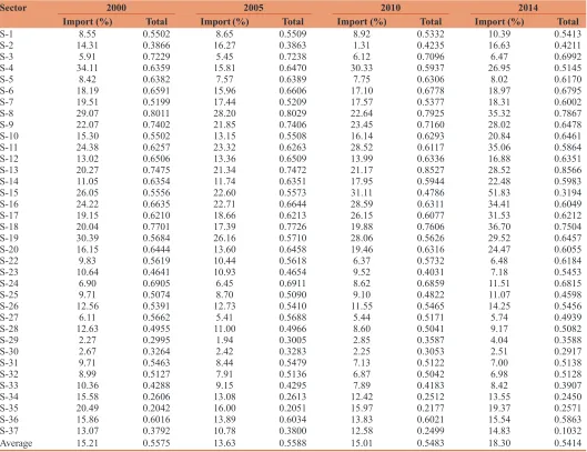
Table 1 provides input coefficients in Australian economy in the year of 2000, 2005, 2010 and 2014. In the year of 2000, input coefficient in Australian economy, on average, was 0.5575. The sector with highest input coefficient was Sector-8 (0.8011) and the sector with smallest input coefficient was Sector-35 (0.2042). The sector with least input coefficient was indicated as the most efficient sector as it needs less input to produce output. Otherwise, the sector with largest input coefficient was indicated as the least efficient sector as it needs highest input to produce output.
In the year of 2005, input coefficients in Australian economy was, on average, 0.5588 a slightly higher than that of the year 2000. The most efficient sector namely the sector with smallest input coefficient was Sector-35 (0.51). The least efficient sector, the sector with highest input coefficient was Sector-8 (0.8029). In the year of 2010, input coefficients in Australian economy was, on average, 0.5483. In the 2010, Australian economy was more efficient than in the year of 2005 as input coefficient was slightly less than that in the year of 2005. The most efficient sector was Sector-35 (0.2177), and the least efficient sector was Sector-13 (0.8527). In the year of 2014, input coefficients was, on average, 0.5414. This year Australian economy as a whole work the most efficient way as input coefficient was the least compared to the year of 2000, 2005, and 2010.
Table 1 also provides import component of input in Australian
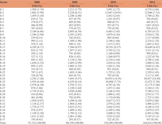
Table 2 provides Australian import of input by sector for the
year of 2000, 2005, 2010 and 2014. In the year of 2000, total Australian import was US$ 47,122 million. Sectorally, the highest import was by Sector-13 (US$ 4,105 million, 8.71%); the smallest import was by Sector-37 (US$ 195 million, 0.41%). Ten highest sectors in import were by Sector-2 (3.99%), Sector-8 (6.66%), Sector-13 (8.71%), Sector-18 (3.52%), Sector-24 (7.20%), Sector-25 (8.44%), Sector-26 (6.30%), Sector-28 (5.81%), Sector-31 (4.07%) and Sector-33 (3.77%). In the year of 2005, total Australian import was US$ 80,358 million. Sectorally, the highest import was by Sector-24 (US$ 7,691 million, 9.57%); the smallest import was by Sector-37 (US$ 293 million, 0.37%). Ten highest sectors in import were by Sector-2 (6.51%), Sector-8 (6.34%), Sector-13 (8.97%), Sector-24 (9.57%), Sector-25 (8.14%), Sector-26 (7.21%), Sector-28 (4.88%), Sector-31 (4.10%), Sector-33 (3.51%), and Sector-36 (3.06%). In the year of 2010, total Australian import was US$ 130, 290 million.
Sectorally, the highest import was by Sector-24 (US$ 18,955 million, 14.55%); the smallest import was by Sector-37 (US$ 322 million, 0.25%). Ten highest sectors in import were by
Sector-2 (10.01%), Sector-8 (3.43%), Sector-13 (8.27%), Sector-24 (14.55%), Sector-25 (7.75%), Sector-26 (6.74%), Sector-28 (3.95%), Sector-31 (3.5%), Sector-33 (2.95%), and Sector-36 (3.02%). In the year of 2014, total Australian import was US$ 164,616 million. Sectorally, the highest import was by Sector-24 (US$ 30,457 million, 18.50%); the smallest import was by Sector-37 (US$ 167 million, 0.10%). Ten highest sectors in import were by Sector-2 (10.01%), Sector-8 (3.43%), Sector-13 (8.27%), Sector-24 (14.55%), Sector-25 (7.75%), Sector-26 (6.74%), Sector-28 (3.95%), Sector-31 (3.5%), Sector-35(3.94%), and Sector-36 (3.13%).
Imports by Sector-2 had steadily increased from 3.99% in 2000 to 6.51% in 2005 and 10.01% in 2010, but declined to 7.32% in 2014. Imports by Sector-8 had declined from 6.66% in 2000 to 6.34% in 2005 and 3.34% in 2010 and so did import by Sector-23, Sector-31
and Sector-33. In percentage, imports by Sector-13 were relatively stable during 2000 to 2010, but a bit declined in 2014. Imports by Sector-24 had increased significantly from 7.20% in 2000 to 9.57% in 2005, 14.55% in 2010 and 18.50% in 2014. Imports by Sector-25 and Sector-26 had been stable during 2000-2014.
Table 1: Import components of input in Australian economy (%): 2000, 2005, 2010, and 2014
Sector 2000 2005 2010 2014
Import (%) Total Import (%) Total Import (%) Total Import (%) Total
S-1 8.55 0.5502 8.65 0.5509 8.92 0.5332 10.39 0.5413
S-2 14.31 0.3866 16.27 0.3863 1.31 0.4235 16.63 0.4211
S-3 5.91 0.7229 5.45 0.7238 6.12 0.7096 6.47 0.6992
S-4 34.11 0.6359 15.81 0.6470 30.33 0.5937 26.95 0.5145
S-5 8.42 0.6382 7.57 0.6389 7.75 0.6306 8.02 0.6170
S-6 18.19 0.6591 15.96 0.6606 17.10 0.6778 18.97 0.6795
S-7 19.51 0.5199 17.44 0.5209 17.57 0.5377 18.31 0.6002
S-8 29.07 0.8011 28.20 0.8029 22.64 0.7925 35.32 0.7867
S-9 22.07 0.7402 21.85 0.7406 23.45 0.7160 28.02 0.6478
S-10 15.30 0.5502 13.15 0.5508 16.14 0.6293 20.84 0.6461
S-11 24.38 0.6257 23.32 0.6263 28.52 0.6117 35.06 0.5864
S-12 13.02 0.6506 13.36 0.6509 13.99 0.6336 16.88 0.6351
S-13 20.27 0.7475 21.34 0.7472 21.17 0.8527 28.52 0.8566
S-14 11.05 0.6354 11.74 0.6351 17.95 0.5944 22.48 0.5983
S-15 26.05 0.5556 22.60 0.5573 31.11 0.4786 51.83 0.3194
S-16 24.22 0.6635 22.71 0.6644 28.59 0.6311 34.41 0.6049
S-17 19.15 0.6210 18.66 0.6213 26.15 0.6077 31.53 0.6212
S-18 20.04 0.7701 17.39 0.7726 19.88 0.7606 36.70 0.7504
S-19 30.39 0.5684 26.16 0.5710 28.06 0.5626 29.52 0.6457
S-20 16.15 0.6444 13.60 0.6458 19.46 0.6316 24.47 0.6055
S-22 9.83 0.5619 10.44 0.5618 6.37 0.5732 6.48 0.6184
S-23 10.64 0.4641 10.93 0.4654 9.52 0.4031 7.18 0.5453
S-24 6.90 0.6905 6.45 0.6911 8.62 0.6859 11.51 0.6815
S-25 9.71 0.5074 8.70 0.5090 9.10 0.4822 11.07 0.4598
S-26 12.56 0.5391 12.73 0.5410 11.55 0.5465 14.25 0.5456
S-27 6.11 0.5662 5.41 0.5688 5.44 0.5171 5.74 0.4939
S-28 12.63 0.4955 11.00 0.4966 8.60 0.5041 9.17 0.5082
S-29 2.27 0.2995 1.94 0.3005 2.85 0.3587 4.04 0.3588
S-30 2.67 0.3264 2.42 0.3283 2.25 0.3053 2.51 0.2917
S-31 9.71 0.5463 8.44 0.5479 7.13 0.5122 7.00 0.5138
S-32 8.99 0.5127 7.91 0.5136 6.87 0.5042 6.98 0.5128
S-33 10.36 0.4288 9.15 0.4295 7.89 0.4183 8.42 0.3907
S-34 15.58 0.2606 13.08 0.2613 12.42 0.2512 13.55 0.2450
S-35 20.49 0.2042 16.00 0.2051 15.97 0.2177 19.37 0.2571
S-36 15.86 0.6016 13.89 0.6034 13.83 0.6021 15.54 0.5863
S-37 13.07 0.3792 10.78 0.3800 12.58 0.2499 14.83 0.1032
Average 15.21 0.5575 13.63 0.5588 15.01 0.5483 18.30 0.5414
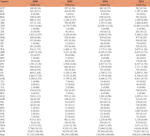
Table 3 provides countries where Australia imported goods and
services (in million US$) for the year of 2000, 2005, 2010 and 2014. In the year of 2000, the highest import came from USA (16.35%), the smallest import came from Bulgaria (0.00%). Out of US$ 47,122 million of Australian import, 1.93% was imported from Canada; 4.06% from China; 3.87% from Germany; 5.28% from UK; 3.36% from Indonesia; 1.84% from Italy; 7.35% from Japan; 2.55% from Korea; 2.91% from Taiwan, 16.35% from USA, and 40.48% from ROW.
In the year of 2005, the highest import came from USA (US$ 9,243 million; 11.50%), the smallest import came from Cyprus (US$ 1 million; 0.00%). Goods and services imported from Canada was US$ 1,346 million (1.67% of total import), from China was US$ 6,379 million (7.94%), from Germany was US$ 3,258 million (4.05%), from UK was US$ 3,521 million (4.38%), from Indonesia was US$ 2,926 million (3.64%), from Italy was US$ 1,520 million (1.89%), from Japan US$4,742 million (5.90%), from Korea US$1,799 million (2.24%), from Taiwan was US$ 2,167 million (2.70%), and from the USA was US$ 9,243 million (11.50%) and the rest US$ 34,870 million (43.39%) was from ROW, rest
of the world. In the year of 2010, the highest import came from China (US$ 16,548 million; 12.70%), the smallest import came from Latvia (US$ 2 million; 0.00%). Goods and services imported from Canada was US$ 1,287 million (0.99%), from Germany was US$ 4,920 million (3.78%), from UK was US$ 4,285 million (3.29%), from Indonesia was US$ 4,837 million (3.71%), from Italy was US$ 1,788 million (1.37%), from Japan US$ 5,738 million (4.40%), from Korea US$ 3,606 million (2.77%), from Taiwan was US$ 2,467 million (1.89%), and from the USA was US$ 12,065 million (9.26%) and the rest US$ 59,364 million (45.56%) was from ROW.
In the year of 2014, the highest import came from China (US$ 23,865 million; 14.50%), the smallest import came from Cyprus as well as from Latvia (US$ 4 million; 0.00%). Goods and services imported from Canada was US$ 1,309 million (0.80 %), from Germany was US$ 5,368 million (3.26%), from UK was US$ 4,475 million (2.72%), from Indonesia was US$ 4,537 million (2.76%), from Italy was US$ 2,569 million (1.56%), from Japan US$ 6,746 million (4.10%), from Korea US$ 6,831 million (4.15%), from Taiwan was US$ 3,671 million (2.23%), and from
Table 2: Australian import of input by sector (million US$): 2000, 2005, 2010 and 2014
Sector 2000 2005 2010 2014
US$ (%) US$ (%) US$ (%) US$ (%)
S-1 1,504 (3.19) 2,211 (2.75) 3,091 (2.37) 4,278 (2.60)
S-2 1,882 (3.99) 5,228 (6.51) 13,047 (10.01) 12,046 (7.32)
S-3 1,459 (3.10) 2,248 (2.80) 3,452 (2.65) 3,780 (2.30)
S-4 810 (1.72) 637 (0.79) 1,261 (0.97) 702 (0.43)
S-5 270 (0.57) 405 (0.50) 480 (0.37) 445 (0.27)
S-6 466 (0.99) 683 (0.85) 932 (0.71) 1,021 (0.62)
S-7 387 (0.82) 579 (0.72) 755 (0.58) 856 (0.52)
S-8 3,140 (6.66) 5,093 (6.34) 4,465 (3.43) 6,795 (4.13)
S-9 1,386 (2.94) 2,291 (2.85) 3,079 (2.36) 2,934 (1.78)
S-10 239 (0.51) 342 (0.43) 865 (0.66) 1,317 (0.80)
S-11 995 (2.11) 1,589 (1.98) 2,190 (1.68) 2,218 (1.35)
S-12 554 (1.18) 949 (1.18) 1,315 (1.01) 1,665 (1.01)
S-13 4,105 (8.71) 7,204 (8.97) 10,781 (8.27) 10,649 (6.47)
S-14 822 (1.75) 1,457 (1.81) 2,745 (2.11) 3,511 (2.13)
S-15 545 (1.16) 791 (0.98) 1,160 (0.89) 999 (0.61)
S-16 527 (1.12) 826 (1.03) 1,260 (0.97) 1,252 (0.76)
S-17 683 (1.45) 1,110 (1.38) 2,134 (1.64) 2,708 (1.64)
S-18 1,656 (3.52) 2,405 (2.99) 2,834 (2.18) 3,880 (2.36)
S-19 695 (1.47) 1,002 (1.25) 1,565 (1.20) 2,042 (1.24)
S-20 333 (0.71) 469 (0.58) 851 (0.65) 844 (0.51)
S-22 787 (1.67) 1,493 (1.86) 1,725 (1.32) 2,359 (1.43)
S-23 328 (0.70) 603 (0.75) 703 (0.54) 3,117 (1.89)
S-24 3,392 (7.20) 7,691 (9.57) 18,955 (14.55) 30,457 (18.50) S-25 3,976 (8.44) 6,539 (8.14) 10,098 (7.75) 12,472 (7.58)
S-26 2,970 (6.30) 5,793 (7.21) 8,787 (6.74) 12,175 (7.40)
S-27 878 (1.86) 1,320 (1.64) 1,872 (1.44) 2,184 (1.33)
S-28 2,739 (5.81) 3,920 (4.88) 5,146 (3.95) 5,780 (3.51)
S-29 414 (0.88) 652 (0.81) 1,890 (1.45) 2,912 (1.77)
S-30 461 (0.98) 792 (0.99) 1,174 (0.90) 1,723 (1.05)
S-31 1,920 (4.07) 3,298 (4.10) 4,657 (3.57) 5,039 (3.06)
S-32 1,118 (2.37) 1,964 (2.44) 2,978 (2.29) 3,406 (2.07)
S-33 1,776 (3.77) 2,823 (3.51) 3,842 (2.95) 4,166 (2.53)
S-34 976 (2.07) 1,489 (1.85) 2,349 (1.80) 3,079 (1.87)
S-35 1,120 (2.38) 1,705 (2.12) 3,600 (2.76) 6,493 (3.94)
S-36 1,611 (3.42) 2,461 (3.06) 3,932 (3.02) 5,147 (3.13)
S-37 195 (0.41) 293 (0.37) 322 (0.25) 167 (0.10)
Total 47,122 (100.00) 80,358 (100.00) 130,290 (100.00) 164,616 (100.00)
the USA was US$ 14,636 million (8.89%) and US$ 72,623 million (44.12%) was from ROW.
During 2000-2014, import from Canada, Japan, UK and the USA had declined significantly. Import from Canada decreased from 1.93% in 2000 to 0.80% in 2014. Import from Japan, decrease from 7.35% in 2000 to 5.90% in 2005, 4.40% in 2010 and 4.10% in 2014. Import from UK decreased from 5.28% in 2000 to 4.38%in 2005, 3.29% in 2010 and 2.72% in 2014. Import from USA decreased from 16.35% in 2000 to 11.50% in 2005, 9.26% in 2010 and 8.89% in 2014. In contrast, import from China increased significantly from 4.06% in 2000 to 7.94% in 2005, to 12.70% in 2010 and to 14.50% in 2014.
Table 4 provides sectoral import multipliers in Australian economy
for the year of 2000 and 2005. Import multipliers were classified
as initial, direct, indirect and total effects of open matrix. Type-1
multiplier is defined as a ratio of total to initial effects.
In the year of 2000, there were some sectors with highest Type-1 import multipliers, namely: Sector-29 (7.9963), Sector-30 (4.6901), Sector-32 (3.3594), Sector-22 (2.7734), Sector-5 (2.7622), Sector-2 (2.7545), and Sector-1 (2.3035. The ratio of total to initial effect was more than 7 times in Sector-29, more than 4 times in Sector-30, more than 3 times in Sector-32. There were
some other sectors with Type-1 import multipliers more than 2,
namely Sector-22 (2.7734), Sector-5 (2.7622), Sector-28 (2.0925), Sector-26 (2.2606), Sector-23 (2.3026), Sector-14 (2.4768), Sector-12 (2.3176), Sector-7 (2.0301), Sector-2 (2.7545) and Sector-1 (2.3035). Other sectors had Type-1 import multipliers <2.
Table 3: Australian import of input by country (million US$): 2000, 2005, 2010 and 2014
Country 2000 2005 2010 2014
US$ (%) US$ (%) US$ (%) US$ (%)
AUT 160 (0.34) 307 (0.38) 481 (0.37) 562 (0.34)
BEL 241 (0.51) 470 (0.59) 736 (0.56) 1,707 (1.04)
BGR 0 (0.00) 7 (0.01) 8 (0.01) 18 (0.01)
BRA 190 (0.40) 460 (0.57) 698 (0.54) 703 (0.43)
CAN 908 (1.93) 1,346 (1.67) 1,287 (0.99) 1,309 (0.80)
CHE 537 (1.14) 794 (0.99) 1,353 (1.04) 1,464 (0,89)
CHN 1,913 (4.06) 6,379 (7.94) 16,548 (12.70) 23,865 (14.50)
CYP 1 (0.00) 1 (0.00) 5 (0.00) 4 (0.00)
CZE 21 (0.05) 92 (011) 165 (0.13) 201 (0.12)
DEU 1,823 (3.87) 3,258 (4.05) 4,920 (3.78) 5,368 (3.26)
DNK 188 (0.40) 358 (0.44) 470 (0.36) 475 (0.29)
ESP 215 (0.46) 452 (0.56) 759 (0.58) 956 (0.58)
EST 1 (0.00) 12 (0.01) 46 (0.04) 79 (0.05)
FIN 281 (0.60) 353 (0.44) 642 (0.49) 526 (0.32)
FRA 816 (1.73) 1,404 (1.75) 1,773 (1.36) 2,075 (1.26)
GBR 2,487 (5.28) 3,521 (4.38) 4,285 (3.29) 4,475 (2.72)
GRC 32 (0.07) 50 (0.06) 44 (0.03) 64 (0.04)
HRV 1 (0.00) 5 (0.01) 4 (0.00) 20 (0.01)
HUN 18 (0.04) 80 (0.10) 121 (0.09) 170 (0.10)
IDN 1,581 (3.36) 2,926 (3.64) 4,837 (3.71) 4,537 (2.76)
IND 304 (0.65) 664 (0.83) 1,159 (0.89) 1,711 (1.04)
IRL 280 (0.59) 344 (0.43) 755 (0.58) 735 (0.45)
ITA 869 (1.84) 1,520 (1.89) 1,788 (1.37) 2,569 (1.56)
JPN 3,462 (7.35) 4,742 (5.90) 5,738 (4.40) 6,746 (4.10)
KOR 1,204 (2.55) 1,799 (2.24) 3,606 (2.77) 6,831 (4.15)
LTU 1 (0.00) 7 (0.01) 14 (0.01) 35 (0.02)
LUX 4 (0.01) 15 (0.02) 36 (0.03) 46 (0.03)
LVA 1 (0.00) 2 (0.00) 2 (0.00) 4 (0.00)
MEX 154 (0.33) 333 (0.41) 584 (0.45) 768 (0.47)
MLT 4 (0.01) 7 (0.01) 4 (0.00) 5 (0.00)
NLD 524 (1.11) 951 (1.18) 1,281 (0.98) 1,829 (1.11)
NOR 88 (0.19) 188 (0.23) 171 (0.13) 314 (0.19)
POL 22 (0.05) 59 (0.07) 163 (0.13) 370 (0.22)
PRT 66 (0.14) 91 (0.11) 76 (0.06) 126 (0.08)
ROU 5 (0.01) 12 (0.01) 20 (0.02) 44 (0.03)
RUS 6 (0.01) 26 (0.03) 315 (0.24) 1,065 (0.65)
SVK 5 (0.01) 12 (0.01) 23 (0.02) 197 (0.12)
SVN 7 (0.02) 25 (0.03) 22 (0.02) 52 (0.03)
SWE 475 (1.01) 861 (1.07) 1,230 (0.94) 1,138 (0.69)
TUR 76 (0.16) 145 (0.18) 224 (0.17) 519 (0.32)
TWN 1,373 (2.91) 2,167 (2.70) 2,467 (1.89) 3,671 (2.23)
USA 7,706 (16.35) 9,243 (11.50) 12,065 (9.26) 14,636 (8.89)
ROW 19,073 (40.48) 34,870 (43.39) 59,364 (45.56) 72,623 (44.12)
Total 47,122 (100.00) 80,358 (100.00) 130,290 (100.00) 164,616 (100.00)
In the year of 2005, there were some sectors with highest Type-1 import multipliers, namely: Sector-29 (8.5114), Sector-30 (4.7530), Sector-32 (3.4031), Sector-31 (2.7346), Sector-5 (2.7449), Sector-22 (2.4919), Sector-2 (2.4569), and Sector-1 (2.2563). The ratio of total to initial effect was more than 8 times in Sector-29, more than 4 times in Sector-30, more than 3 times in Sector-32. There were
some other sectors with Type-1 import multipliers more than 2, namely
Sector-31 (2.7346), Sector-5 (2.7449), Sector-22 (2.4919), Sector-28, Sector-26, Sector-23, Sector-14 (2.2310), Sector-12 (2.1280), Sector-7, Sector-2 (2.4569) and Sector-1. Other sectors had Type-1 import multipliers <2.
During the year of 2000-2005, Sector-29, Sector-30, Sector-32, Sector-22, Sector-5, Sector-28, Sector-26, Sector-23, Sector-14, Sector-12, Sector-7, Sector-2, and Sector-1 have consistently had
high import multipliers.
Table 5 provides sectoral import multipliers in Australian economy for the year of 2010 and 2014. In the year of 2010, there were sectors that had Type-1 import multipliers more than 2, namely: Sector-1 (2.1714), Sector-2 (2.1073), Sector-5 (3.05167), Sector-12 (2.2585), Sector-22 (3.3794),
Sector-23 (2.5141), Sector-26 (2.1851), Sector-28 (2.3845), Sector-29 (5.6782), Sector-30 (5.0062), Sector-31 (3.2356), and Sector-32 (3.7109). Increasing final demand in these sectors would increase total import more than twice. Even, in Sector-29, and Sector-30, would increase total import more than 5 times
to initial imports.
In the year of 2014, there were sectors with type-1 import multipliers more than 2, namely: Sector-1 (2.1132), Sector-5 (3.4480), Sector-12 (2.3590), Sector-22 (4.3548), Sector-26 (2.0473), Sector-28 (2.4475), Sector-29 (4.9308), Sector-30 (4.9765), Sector-31 (3.5979), and Sector-32 (3.8593). Increasing final
demand in these sectors would increase total import more than
twice. Even, in Sector-22, Sector-29, and Sector-30 Type-1 import multipliers were more than 4; meaning that the ratio between total
effects and initial effects were more than 4 times.
Table 6 provides country-import multipliers in Australian economy:
Initial, direct, indirect and total effects, for the year 2000, 2005, 2010 and 2014. In average, Type-1 country-import multipliers in Australian economy were: 1.9435, 1.9580, 1.9409 and 1.8867 consecutively for the year of 2000, 2005, 2010 and 2014.
Table 4: Disaggregated import multipliers by sector in Australian Economy, 2000 and 2005
Sector 2000 2005
Initial Direct Indirect Total Type-1 Initial Direct Indirect Total Type-1
S-1 0.0019 0.0013 0.0012 0.0044 2.3035 0.0015 0.0010 0.0009 0.0034 2.2563
S-2 0.0024 0.0026 0.0015 0.0065 2.7545 0.0035 0.0032 0.0019 0.0087 2.4569
S-3 0.0018 0.0008 0.0006 0.0033 1.7954 0.0015 0.0007 0.0005 0.0027 1.7907
S-4 0.0010 0.0001 0.0000 0.0011 1.1276 0.0004 0.0002 0.0001 0.0007 1.6910 S-5 0.0003 0.0003 0.0003 0.0009 2.7622 0.0003 0.0003 0.0002 0.0007 2.7449
S-6 0.0006 0.0003 0.0002 0.0011 1.7969 0.0005 0.0002 0.0002 0.0008 1.8291 S-7 0.0005 0.0003 0.0002 0.0010 2.0301 0.0004 0.0002 0.0002 0.0008 2.0332
S-8 0.0039 0.0008 0.0008 0.0056 1.4078 0.0034 0.0007 0.0007 0.0048 1.4130 S-9 0.0017 0.0008 0.0006 0.0031 1.7743 0.0015 0.0006 0.0005 0.0027 1.7506 S-10 0.0003 0.0001 0.0001 0.0005 1.6109 0.0002 0.0001 0.0001 0.0004 1.7399
S-11 0.0013 0.0005 0.0004 0.0022 1.7271 0.0011 0.0004 0.0003 0.0018 1.6753
S-12 0.0007 0.0005 0.0004 0.0016 2.3176 0.0006 0.0004 0.0003 0.0014 2.1280
S-13 0.0052 0.0019 0.0013 0.0083 1.6182 0.0049 0.0018 0.0012 0.0079 1.6259
S-14 0.0010 0.0008 0.0007 0.0026 2.4768 0.0010 0.0007 0.0005 0.0022 2.2310 S-15 0.0007 0.0001 0.0001 0.0009 1.2850 0.0005 0.0001 0.0001 0.0007 1.3173
S-16 0.0007 0.0001 0.0001 0.0009 1.3203 0.0006 0.0001 0.0001 0.0007 1.3046 S-17 0.0009 0.0002 0.0002 0.0013 1.4676 0.0007 0.0002 0.0001 0.0011 1.4093
S-18 0.0021 0.0004 0.0002 0.0027 1.2880 0.0016 0.0003 0.0002 0.0022 1.3316
S-19 0.0009 0.0001 0.0001 0.0011 1.2728 0.0007 0.0001 0.0001 0.0009 1.3223
S-20 0.0004 0.0001 0.0001 0.0006 1.4902 0.0003 0.0001 0.0001 0.0005 1.5409
S-22 0.0010 0.0009 0.0009 0.0027 2.7734 0.0010 0.0008 0.0007 0.0025 2.4919
S-23 0.0004 0.0003 0.0003 0.0009 2.3026 0.0004 0.0002 0.0002 0.0009 2.1615
S-24 0.0043 0.0018 0.0016 0.0076 1.7823 0.0052 0.0021 0.0018 0.0091 1.7482 S-25 0.0050 0.0025 0.0021 0.0096 1.9167 0.0044 0.0022 0.0018 0.0084 1.9116
S-26 0.0037 0.0024 0.0023 0.0084 2.2606 0.0039 0.0023 0.0023 0.0085 2.1760 S-27 0.0011 0.0003 0.0003 0.0017 1.5098 0.0009 0.0002 0.0002 0.0014 1.5284
S-28 0.0034 0.0019 0.0019 0.0072 2.0925 0.0026 0.0014 0.0015 0.0056 2.1030 S-29 0.0005 0.0014 0.0022 0.0042 7.9963 0.0004 0.0013 0.0020 0.0037 8.5114 S-30 0.0006 0.0010 0.0012 0.0027 4.6901 0.0005 0.0009 0.0011 0.0025 4.7530
S-31 0.0024 0.0020 0.0021 0.0065 2.6992 0.0022 0.0018 0.0020 0.0061 2.7346
S-32 0.0014 0.0017 0.0016 0.0047 3.3594 0.0013 0.0016 0.0016 0.0045 3.4031
S-33 0.0022 0.0004 0.0004 0.0030 1.3540 0.0019 0.0004 0.0004 0.0026 1.3771
S-34 0.0012 0.0001 0.0001 0.0015 1.1842 0.0010 0.0001 0.0001 0.0012 1.2189 S-35 0.0014 0.0000 0.0000 0.0014 1.0295 0.0011 0.0000 0.0000 0.0012 1.0384
S-36 0.0020 0.0005 0.0005 0.0030 1.4974 0.0017 0.0004 0.0005 0.0025 1.5262 S-37 0.0002 0.0000 0.0000 0.0003 1.3278 0.0002 0.0000 0.0000 0.0003 1.3707
In the year of 2000, the highest Type-1 import multiplier was import from Canada (2.0213), followed by import from Italy (1.985). The smallest Type-1 import multiplier was import from the USA (1.9022). Increasing final demand in Australia by 1%, initially increased import from the USA by 0.0097%, directly increased import from the USA by 0.0046%, indirectly increased import from the USA by 0.0130%, resulting total effect to 0.0184%. There was no significant different by country of import origin, in term Type-1 import multipliers. In the year of 2005, the highest Type-1 import multiplier was import from Italy (2.0120), followed by import from France (2.0019). The smallest Type-1 import multiplier was import from Germany (1.9260). Increasing final demand in Australia by 1%, initially increased import from Germany by 0.0022%, directly increased import from Germany by 0.0011%, indirectly increased import from Germany by 0.0011%, resulting total effect to Australian import by 0.0044%. Again, in the year of 2005, there was no significant different by country of
import origin, in term Type-1 import multipliers.
In the year of 2010, the highest Type-1 import multiplier was import from Indonesia (2.0122) and the smallest Type-1 import multiplier was import from Germany (1.8994). In the year 2010,
there were no significant different Type-1 import multipliers based on the country of import origin. In the year of 2014, the highest Type-1 import multiplies was import from Indonesia (1.9407) and
the smallest Type-1 import multiplier was import from Germany
(1.8474). In the year of 2014, there were no significant different
Type-1 import multipliers based on the country of import origin.
5. CONCLUSION
From discussion above, some conclusion could be drawn. Firstly,
Australian import components of input were, on average, <20%; meaning that input that locally provided were more than 80%. Australian import of input had increased significantly from US$ 47,122 million in 2000 to US$ 14,616 million in 2014.
Secondly, Australian imports have been dominated by S-13:
Manufacture of basic metals, S-25: Wholesale and retail trade and repair, S-24: Construction, S-8: Manufacture of coke and refined
petroleum products, and S-26: Transportation and post services.
Thirdly, by country of origin, Australian imports have been dominated by the USA, Japan, United Kingdom, China and
Table 5: Disaggregated import multipliers by sector in Australian Economy, 2010 and 2014
Sector 2010 2014
Initial Direct Indirect Total Type-1 Initial Direct Indirect Total Type-1
S-1 0.0012 0.0008 0.0007 0.0027 2.1714 0.0015 0.0009 0.0008 0.0032 2.1132 S-2 0.0053 0.0037 0.0021 0.0111 2.1073 0.0043 0.0025 0.0010 0.0078 1.8105
S-3 0.0014 0.0005 0.0004 0.0023 1.6643 0.0014 0.0005 0.0004 0.0023 1.6695
S-4 0.0005 0.0001 0.0000 0.0006 1.2409 0.0003 0.0000 0.0000 0.0003 1.3021 S-5 0.0002 0.0002 0.0002 0.0006 3.0167 0.0002 0.0002 0.0002 0.0006 3.4880
S-6 0.0004 0.0001 0.0001 0.0006 1.6969 0.0004 0.0001 0.0001 0.0006 1.6645 S-7 0.0003 0.0002 0.0001 0.0006 1.9873 0.0003 0.0001 0.0001 0.0006 1.9254
S-8 0.0018 0.0004 0.0004 0.0027 1.4819 0.0024 0.0005 0.0004 0.0033 1.3472 S-9 0.0012 0.0004 0.0003 0.0020 1.5810 0.0011 0.0003 0.0002 0.0016 1.5093 S-10 0.0003 0.0001 0.0001 0.0005 1.4685 0.0005 0.0001 0.0001 0.0007 1.3884 S-11 0.0009 0.0003 0.0002 0.0014 1.5368 0.0008 0.0002 0.0001 0.0012 1.4703
S-12 0.0005 0.0004 0.0003 0.0012 2.2585 0.0006 0.0005 0.0003 0.0014 2.3590
S-13 0.0043 0.0011 0.0006 0.0061 1.4039 0.0038 0.0008 0.0004 0.0050 1.3180
S-14 0.0011 0.0006 0.0004 0.0021 1.9077 0.0013 0.0006 0.0004 0.0023 1.8491 S-15 0.0005 0.0001 0.0001 0.0006 1.2633 0.0004 0.0001 0.0000 0.0005 1.3157
S-16 0.0005 0.0001 0.0001 0.0007 1.3357 0.0004 0.0001 0.0001 0.0007 1.4977 S-17 0.0009 0.0002 0.0001 0.0012 1.3492 0.0010 0.0003 0.0002 0.0014 1.4874
S-18 0.0011 0.0003 0.0002 0.0016 1.4318 0.0014 0.0002 0.0001 0.0017 1.1878 S-19 0.0006 0.0001 0.0001 0.0008 1.3014 0.0007 0.0001 0.0001 0.0010 1.2971 S-20 0.0003 0.0001 0.0001 0.0005 1.4068 0.0003 0.0001 0.0000 0.0004 1.3596
S-22 0.0007 0.0008 0.0009 0.0023 3.3794 0.0008 0.0013 0.0015 0.0037 4.3548
S-23 0.0003 0.0002 0.0002 0.0007 2.5141 0.0011 0.0003 0.0002 0.0016 1.4474
S-24 0.0076 0.0028 0.0022 0.0126 1.6542 0.0109 0.0039 0.0028 0.0177 1.6163
S-25 0.0041 0.0020 0.0016 0.0077 1.9023 0.0045 0.0022 0.0016 0.0083 1.8613 S-26 0.0035 0.0021 0.0020 0.0077 2.1851 0.0044 0.0024 0.0021 0.0090 2.0473 S-27 0.0008 0.0002 0.0002 0.0012 1.5985 0.0008 0.0003 0.0003 0.0013 1.6734
S-28 0.0021 0.0013 0.0016 0.0049 2.3845 0.0021 0.0013 0.0017 0.0051 2.4475 S-29 0.0008 0.0014 0.0022 0.0043 5.6782 0.0010 0.0017 0.0024 0.0052 4.9308 S-30 0.0005 0.0008 0.0010 0.0024 5.0062 0.0006 0.0011 0.0013 0.0031 4.9765
S-31 0.0019 0.0020 0.0022 0.0061 3.2356 0.0018 0.0022 0.0025 0.0065 3.5979
S-32 0.0012 0.0016 0.0017 0.0044 3.7109 0.0012 0.0017 0.0018 0.0047 3.8593
S-33 0.0015 0.0003 0.0003 0.0022 1.4356 0.0015 0.0004 0.0002 0.0021 1.4119
S-34 0.0009 0.0001 0.0001 0.0011 1.1796 0.0011 0.0001 0.0001 0.0013 1.1561 S-35 0.0014 0.0000 0.0000 0.0015 1.0480 0.0023 0.0000 0.0000 0.0024 1.0376
S-36 0.0016 0.0004 0.0005 0.0025 1.5728 0.0018 0.0006 0.0005 0.0030 1.5965 S-37 0.0001 0.0000 0.0000 0.0002 1.4127 0.0001 0.0000 0.0000 0.0001 1.7892
Germany. During 2000-2014, import from Canada, Japan, UK and the USA had declined but import from China had significantly
increased. Finally, highest sectoral import multipliers occurred if
final demands change in S-5: Manufacture of wood and of products
of wood and cork, except furniture, S-22: Electricity, gas, steam
and air conditioning supply, S-29: Financial, pension funding and insurance services, S-30: Real estate activities, S-31: Legal and management consultancy, architectures and engineering, scientific
research and development, and S-32: Administrative and support
service activities, but there was no significant different of import
multipliers for country origin of import.
REFERENCES
Ahiakpor, J.C.W. (2000), Hawtrey on the Keynesian multiplier: A question of cognitive dissonance? History of Political Economy, 32(4), 889-908. Beemiller, R.M. (1990), Improving accuracy by combining primary data
with RIMS: Comment on Bourque. International Regional Science
Review, 13(1-2), 99-101.
Burda, W. (2005), Macroeconomics: A European Text. 4th ed. Oxford: Oxford University Press.
Coughlin, C., Mandelbaum, T.B. (1991), A Consumer’s Guide to Regional
Economic Multipliers. Federal Reserve Bank of St. Louis Review.
p19-32.
Dornbusch, R., Stanley, F. (1994), Macroeconomics. 6th ed. International edition. New York: McGraw-Hill.
Grady, P., Muller, R.A. (1988), On the use and misuse of input-output
based impact analysis in evaluation. The Canadian Journal of
Program Evaluation, 2(3), 49-61.
Hall, R.E. (2009), By How Much Does GDP Rise if the Government Buys More Output? NBER Working Paper 15496. National Bureau of Economic Research. Available from: http://www.nber.org/papers/ w15496.pdf?new_window=1.
Harris, P. (1997), Limitations on the use of regional economic impact
multipliers by practitioners: An application to the tourism industry.
The Journal of Tourism Studies, 8(2), 1-12.
Hughes, D.W. (2003), Policy Uses of Economic Multipliers and Impact
Analysis. Choices Publication of the American Agricultural
Economics Association, Second Quarter. Available from: http:// www.choicesmagazine.org/2003-2/2003-2-06.htm.
Isard, W. (1951), Inter-regional and Regional Input-Output Analysis:
A Model of a Space-Economy. Review of Economics and Statistics,
33(4), 318-328.
Jensen, R.C., Mandeville, T.D., Karunaratne, N.D. (1979), Regional
Economic Planning: Generation of Regional Input-Output Analysis. London: Croom Helm.
Joshi, R.M. (2009), International Business. New Delhi, New York: Oxford
University Press.
Kahn, R. (1931), The relation of home investment to unemployment. Economic Journal, 41(162), 173-198.
Krugman, P., Wells, R. (2009), Economics. Duffield, UK: Worth Publisher. Leontief, W.W. (1951), The Structure of American Economy 1919-1939.
2nd ed. Cambridge: Harvard University Press.
Lequiller, F., Blades, D. (2006), Understanding National Accounts. Paris: OECD. p139-143. Available from: http://www.oecd.org/std/ UNA-2014.pdf.
Mankiw, N.G. (2008), Macroeconomics. 8th ed. Ohio, USA: South-Western Publishing.
McConnell, C., Brue, S., Flynn, S. (2011), Macroeconomics. 19th ed. New York: McGraw-Hill Series Economics.
Table 6: Import multipliers by country in Australian Economy, 2000, 2005, 2010, and 2014
Country 2000 2005
Initial Direct Indirect Total Type-1 Initial Direct Indirect Total Type-1
CAN 0.0011 0.0006 0.0006 0.0023 2.0213 0.0009 0.0005 0.0004 0.0018 1.9894
CHN 0.0024 0.0012 0.0011 0.0046 1.9306 0.0043 0.0022 0.0020 0.0085 1.9727
DEU 0.0023 0.0011 0.0011 0.0045 1.9610 0.0022 0.0011 0.0011 0.0044 1.9883
FRA 0.0010 0.0005 0.0005 0.0020 1.9708 0.0009 0.0005 0.0005 0.0019 2.0019
GBR 0.0031 0.0015 0.0014 0.0060 1.9060 0.0024 0.0011 0.0011 0.0046 1.9260
IDN 0.0020 0.0010 0.0009 0.0039 1.9862 0.0020 0.0010 0.0009 0.0039 1.9856
ITA 0.0011 0.0006 0.0005 0.0022 1.9857 0.0010 0.0005 0.0005 0.0021 2.0120
JPN 0.0044 0.0022 0.0020 0.0085 1.9603 0.0032 0.0016 0.0015 0.0063 1.9846
KOR 0.0015 0.0008 0.0007 0.0030 1.9688 0.0012 0.0006 0.0006 0.0024 1.9828
TWN 0.0017 0.0008 0.0008 0.0033 1.9294 0.0015 0.0007 0.0007 0.0029 1.9629
USA 0.0097 0.0046 0.0042 0.0184 1.9022 0.0062 0.0030 0.0028 0.0120 1.9281
ROW 0.0289 0.0145 0.0130 0.0563 1.9495 0.0283 0.0142 0.0127 0.0553 1.9521
TOTAL 0.0592 0.0292 0.0266 0.1151 1.9435 0.0541 0.0271 0.0248 0.1060 1.9580
Country 2010 2014
Initial Direct Indirect Total Type-1 Initial Direct Indirect Total Type-1
CAN 0.0005 0.0003 0.0002 0.0010 1.9331 0.0005 0.0002 0.0002 0.0009 1.8873
CHN 0.0067 0.0032 0.0030 0.0128 1.9230 0.0086 0.0040 0.0036 0.0161 1.8831 DEU 0.0020 0.0010 0.0009 0.0039 1.9521 0.0019 0.0009 0.0008 0.0036 1.8916
FRA 0.0007 0.0004 0.0003 0.0014 1.9592 0.0007 0.0004 0.0003 0.0014 1.8879
GBR 0.0017 0.0008 0.0007 0.0033 1.8994 0.0016 0.0007 0.0006 0.0030 1.8474
IDN 0.0019 0.0010 0.0009 0.0039 2.0122 0.0016 0.0008 0.0007 0.0032 1.9407
ITA 0.0007 0.0004 0.0003 0.0014 1.9583 0.0009 0.0004 0.0004 00018 1.9030
JPN 0.0023 0.0011 0.0011 0.0045 1.9553 0.0024 0.0012 0.0010 0.0046 1.8977
KOR 0.0015 0.0007 0.0007 0.0028 1.9437 0.0025 0.0012 0.0010 0.0047 1.9020
TWN 0.0010 0.0005 0.0005 0.0019 1.9434 0.0013 0.0006 0.0006 0.0025 1.8879
USA 0.0049 0.0023 0.0021 0.0092 1.9005 0.0053 0.0024 0.0021 0.0097 1.8535
ROW 0.0286 0.0143 0.0127 0.0556 1.9466 0.0318 0.0152 0.0131 0.0601 1.8894
TOTAL 0.0524 0.0259 0.0234 0.1018 1.9409 0.0592 0.0280 0.0244 0.1116 1.8867
Miller, R., Blair, P. (1985), Input-Output Analysis-Foundations and
Extensions. New Jersey: Prentice-Hall, Englewood Cliffs.
Mills, E.C. (1993), The misuse of regional economic models. Cato Journal, 13(1), 29-39.
Moore, F.T., Petersen, J. (1955), Regional analysis: An inter-industry model of Utah. Review of Economics and Statistics, 37, 368-383. Muchdie, M. (2017), Technical and trade coefficients in indonesian and
australian economies: A comparison. Global Journal for Research
Analysis, 6(11), 290-296.
Oosterhaven, J., Stelder, D. (2007), Regional and Interregional IO
Analysis. The Netherlands: Faculty of Economics and Business
University of Groningen. Available from: https://www.rug.nl/ research/reg/research/irios/download/regional-io-analysis.pdf. Pindyck, R., Rubinfeld, D. (2012), Macroeconomics. The Pearson Series
in Economics. 8th ed. London: Pearson.
Richardson, H.W. (1985), Input-output and economic base multipliers: Looking backward and forward. Journal of Regional Science, 25(4), 607-661.
Siegfried, J., Allen, R., Sanderson, A.R., McHenry, P. (2006), The Economic Impact of Colleges and Universities. Working Paper No. 06-W12. Available from: http://www.accessecon.com/pubs/VUECON/vu06-w12.pdf. Tiebout, C.M. (1956), A pure theory of local expenditures. The Journal
of Political Economy, 64(5), 416-424.
Timmer, M.P., Dietzenbacher, E., Los, B., Stehrer, R., de Vries, G.J.
(2015), An illustrated user guide to the world input-output database:
The Case of Global Automotive Production. Review of International
Economics, 23(3), 575-605.
Timmer, M.P., Los, B., Stehrer, R, de Vries, G.J. (2016), An Anatomy of the Global Trade Slowdown based on the WIOD 2016 Release.
GGDC Research Memorandum Number 162, University of
Groningen. Available from: http://www.ggdc.net/publications/ memorandum/gd162.pdf.
Trinh, B., Hoa, P.L., Giang, B.C. (2008), Import Multiplier in Input-Output Analysis. Depocen Working Paper Series No. 2008/23.
West, G.R. (1990), Regional trade estimation: A hybrid approach. International Regional Science Review, 13(1-2), 103-118.
Appendix 1: Sector classifications
Sector code Descriptions
Sector-1 Crop and animal production, forestry, fishing and aquaculture
Sector-2 Mining and quarrying
Sector-3 Manufacture of food products, beverages and tobacco products
Sector-4 Manufacture of textiles, wearing apparel and leather products
Sector-5 Manufacture of wood and of products of wood and cork, except furniture
Sector-6 Manufacture of paper and paper products
Sector-7 Printing and reproduction of recorded media
Sector-8 Manufacture of coke and refined petroleum products
Sector-9 Manufacture of chemicals and chemical products
Sector-10 Manufacture of basic pharmaceutical products and pharmaceutical preparations
Sector-11 Manufacture of rubber and plastic products
Sector-12 Manufacture of other non-metallic mineral products
Sector-13 Manufacture of basic metals
Sector-14 Manufacture of fabricated metal products, except machinery and equipment
Sector-15 Manufacture of computer, electronic and optical products
Sector-16 Manufacture of electrical equipment
Sector-17 Manufacture of machinery and equipment n.e.c
Sector-18 Manufacture of motor vehicles, trailers and semi-trailers
Sector-19 Manufacture of other transport equipment
Sector-20 Manufacture of furniture; other manufacturing
Sector-21 Other manufacturing
Sector-22 Electricity, gas, steam and air conditioning supply
Sector-23 Water collection, sewerage; waste collection, treatment and disposal activities
Sector-24 Construction
Sector-25 Wholesale and retail trade and repair
Sector-26 Transportation and post services
Sector-27 Accommodation and food service activities
Sector-28 Telecommunications, information and publication
Sector-29 Financial, pension funding and insurance services
Sector-30 Real estate activities
Sector-31 Legal and management, architectures and engineering, research and development
Sector-32 Administrative and support service activities
Sector-33 Public administration and defense; compulsory social security
Sector-34 Education
Sector-35 Human health and social work activities
Sector-36 Other service activities
Sector-37 Activities of households as employers Source: Aggregated from WIOT, 2017
Appendix 2: Country abbreviations
No. Acronym Country
included No. Acronym Country included
1. AUS Australia 23. IRL Ireland
2. AUT Austria 24. ITA Italy
3. BEL Belgium 25. JPN Japan
4. BGR Bulgaria 26. KOR Korea
5. BRA Brazil 27. LTU Lithuania
6. CAN Canada 28. LUX Luxembourg
7. CHE Switzerland 29. LVA Latvia
8. CHN China 30. MEX Mexico
9. CYP Cyprus 31. MLT Malta
10 CZE Czech
Republic 32. NLD Netherlands
11. DEU Germany 33. NOR Norway
12. DNK Denmark 34. POL Poland
13. ESP Spain 35. PRT Portugal
14. EST Estonia 36. ROU Romania
15. FIN Finland 37. RUS Russia
16. FRA France 38. SVK Slovak
Republic
17. GBR United
Kingdom 39. SVN Slovenia
18. GRC Greece 40. SWE Sweden
19. HRV Croatia 41. TUR Turkey
20. HUN Hungary 42. TWN Taiwan
21. IDN Indonesia 43. USA United
States
22. IND India 44. ROW Rest of the