JIEM, 2017 – 10(5): 817-852 – Online ISSN: 2013-0953 – Print ISSN: 2013-8423 https://doi.org/10.3926/jiem.2321
Assessing Location Attractiveness for Manufacturing Automobiles
Edward Hanawalt , William Rouse
General Motors, Stevens Institute of Technology (United States)
edward.hanawalt@gm.com, wrouse@stevens.edu
Received: April 2017 Accepted: July 2017
Abstract:
Purpose: Evaluating country manufacturing location attractiveness on various performance measures deepens the analysis and provides a more informed basis for manufacturing site selection versus reliance on labor rates alone. A short list of countries can be used to drive regional considerations for site-specific selection within a country.
Design/methodology/approach: The two-step multi attribute decision model contains an initial filter layer to require minimum values for low weighted attributes and provides a rank order utility score for twenty-three countries studied. The model contains 11 key explanatory variables with Labor Rate, Material Cost, and Logistics making up the top 3 attributes and representing 54% percent of the model weights.
Findings: We propose a multi attribute decision framework for strategically assessing the attractiveness of a country as a location for manufacturing automobiles.
Research limitations/implications: Consideration of country level wage variation, specific tariffs, and other economic incentives provides a secondary analysis after the initial list of candidate countries is defined.
Originality/value: Combining MAUT with regression analysis to simplify model to core factors then using a “must have” layer to handle extreme impacts of low weight factors and allowing for ease of repeatability.
Keywords: automobile, manufacturing, attractiveness, decision making, footprint, optimization, site selection
1. Introduction
The question of where to manufacture and sell goods is paramount for any durable goods manufacturer. Expanding sales into global markets or stretching a supply chain to provide goods from factories thousands of miles away impacts not only the bottom line of an enterprise, but also increases financial and supply chain risks and a companies’ brand image. In “Car Wars”, we discussed the factors driving product success and failure in the automotive market from a product perspective (Hanawalt & Rouse, 2010). “Car Wars” evaluated success or failure in the United States only. However, today’s decisions for durable goods manufacturers are predominately global in nature. Once a product has been planned for development, often the next step is to determine where to sell it and where to build it. While integrated product development processes do most of this work in parallel today, extension of sales into additional markets to further spread out fixed costs or the creation of additional manufacturing footprints is still a very common exercise.
2. Traditional Manufacturing Allocations
The traditional mindset of manufacturers has always been to seek the lowest labor costs in manufacturing location selection. However, the lowest labor cost does not always prove to the best choice for the company in terms of financial returns or risks to a firm’s reputation. The decision to manufacture in a country is a long-term commitment by a company, often 20 years without incurring any financial penalties in terms of write downs of assets or the refunding of government incentives. A wrong bet can transform what should be a competitive advantage into a mess of underutilized or high-cost assets (Lamarre, Pergler & Vainberg, 2009). Much has been written about the outsourcing and insourcing of manufacturing jobs over the last two decades. BCG recently issued a report citing the shifting economics of global manufacturing which identified a trend away from pure low cost manufacturing locations (The Boston Consulting Group, 2014). Manufacturing location selection is much more complicated than purely seeking a country with the lowest labor costs. The location decision needs to be evaluated over various performance measures to ensure a robust decision. Often the high growth potential of an emerging market prompts businesses to invest in order to capitalize on the growth. But too often, as has been the case in India, the results are only news of scams, cases of graft, endemic corruption, enforcement and whistle-blowers (EY, 2014). The stability of the local governments impact manufacturers when issues such as foreign exchange controls can grind production to a halt when dollars are not available to import raw materials, as has been the case in Egypt (Voice of America, 2016).
3. Literature Review
exchange rate through mixed integer programming (Vidal & Goetschalckx, 2000). Dogan proposes an integrated approach that combines Bayesian Networks and Total Cost of Ownership (TCO) to address complexities involved in selecting an international facility for a manufacturing plant (Dogan, 2012).
Alternative approaches have employed survey data and decision frameworks to arrive at an ideal selection. Ellram evaluated country attractiveness through a survey approach with a supply chain focus (Ellram, 2013). Tate and colleagues applied a survey approach, with survey responses from 319 companies currently managing offshore manufacturing plants, to understand attitudes on manufacturing location selection (Tate, Ellram, Schoenherr, & Petersen, 2014). Yang presents an AHP (analytical hierarchy process) decision model for facility location selection from the view of organizations that contemplate locations of a new facility or a relocation of existing facilities (Yang & Lee, 1997). Canboleat et al present a multi-phase approach for selecting a country in which to locate a global manufacturing facility using influence diagrams, decision trees, and a MAUT (multi-attribute utility theory) model (Canbolat, Chelst & Garg, 2007).
The decision to locate a manufacturing facility in a given country must consider both qualitative factors and quantitative factors (MacCormack, Newman III & Rosenfield, 1994). Multi-criteria decision models have been used in a wide range of facility context decisions. Keeney discusses how decisions involving multiple objectives have many factors affecting the desirability of an alternative (Keeney, 1982). Defining a global manufacturing strategy is a very complicated process involving multiple objectives that is evolving away from decision making based on lowest cost alone. Platts used utility theory in the strategic framing and analysis of make vs buy decisions (Platts, 2002). Min proposes a MAUT model for international supplier selection that can effectively deal with both qualitative and quantitative factors in multiple criteria and uncertain decision environments (Min, 1994).
4. Fundamental Objective Hierarchy
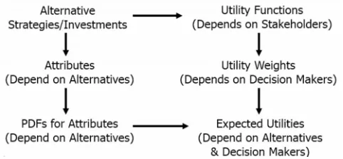
The fundamental objective and supporting objectives of our decision framework are shown in Figure 1.
The fundamental objective hierarchy identifies the decision to be taken and the supporting objectives to arrive at the ideal solution. The fundamental objective defines what is truly wanted from the decision. The supporting objectives are means to achieve the fundamental objective. The fundamental objectives hierarchy creates the framework for measuring alternatives against key attributes.
Figure 1. Fundamental objectives hierarchy
5. Means Objective Network
The means objectives support the achievement of the fundamental objective. Figure 2 shows the means objective network for the decision model.
Working through the Means Objective Network, two primary supporting objectives were identified: Lowest Landed Cost and Minimize Production Risk. Lowest Landed Cost is defined as the lowest cost possible to produce a complete vehicle in a country and Minimize Production Risk is defined as working to prevent interruption of manufacturing production.
6. Decision Framework
6.1. Objective
To evaluate allocation decisions beyond wage rates, we have created a framework that trades off competing attributes to deliver a simple country ranking scale. The goal of the framework is to provide an efficient and repeatable ranking scale. The scale uses reliable data inputs from established sources, some publically available and some purchased. The use of the framework efficiently allows an analyst to very quickly narrow to a small set of candidate countries rather than performing a full-scale site selection study for many countries. Candidate countries can be used to narrow regional considerations within a country and ultimately narrow to a final manufacturing site selection.
Our country attractiveness decision framework employs utility theory as a basis for analysis. The best course of action, or in this case the best country to manufacture in, is the alternative with the highest expected utility. The model employs converted multiple performance measures to a scalar performance measure using multi-attribute utility theory (Keeney & Raiffa, 1993). Each measure requires a utility function complete with relative weighting of importance. The performance measures are converted from their individual native units into utility values. The scores are cardinal and can be used for ranking. Great care is taken to ensure that the decision maker preferences are accurately represented. The following steps were undertaken to create the country attractiveness model:
1. Brainstorm attributes
2. Weight attributes
3. Locate source data for attributes
4. Assign utility functions
5. Score initial set of countries
6. Regression analysis to reduce attributes
7. Review results
8. Sensitivity Analyses
6.1.1. Brainstorm Attributes
A team of ten stakeholders in automotive manufacturing strategy and planning convened in three one-hour sessions to create a listing of potential model attributes for manufacturing country attractiveness. During the first session, an initial set of categories was agreed upon. The broader attribute categories included Automotive, Financial/Macroeconomic, Infrastructure, Investment, Labor, Political, Productivity, and Technology. The next two sessions were used to develop attributes in each of the broad categories. The sessions produced a listing of 25 model attributes to be weighted. The list of broad categories and attributes with each category is the following:
Automotive – Attributes specific to automotive industry, such as metrics on future automotive sales in specific countries.
• Forecasted Production Compound Annual Growth Rate (CAGR%) – Forecasted Automotive Production Growth Rate by country (CY2012 -2018)
• Forecasted market sales CAGR% – Forecasted Automotive Sales Growth Rate by country (CY2012 -2018)
• Material Cost – Relative cost of automotive materials by country, forecasted in 2018
Financial/Macroeconomic – Attributes covering macroeconomic financial metrics, such as inflation rate and consumer price index
• Inflation, consumer prices (annual %) – Rate of inflation by country (average of CY2012-2014) • Foreign Exchange variation – Variability in currency value relative to USD (standard deviation of
% change from '97-13)
• Macroeconomic environment – Stability of the macroeconomic environment (index value) • Value add in MFG – Value added (% of GDP) (average of CY2012-2014)
Infrastructure – Attributes specific to infrastructure metrics, such as electricity prices and logistics performance
• Electricity Price Index – Base electricity rate indexed to UK Base Electricity: Index (2005 = 100) (index value 2014)
• Local Supplier Quality – Quality of local suppliers (index value 2014) • Logistics – Rating of countries logistics capabilities (index value 2014)
• Quality of Electric supply – Rating of countries power supply (index value 2014)
Investment – Attributes specific to investment metrics, such as foreign direct investment in a specific country
• Legal Rights Index – Degree of legal protection of borrowers’ and lenders’ rights (index value 2014)
Labor – Attributes specific to labor metrics, such as labor rate and quality of education system
• Labor Market Efficiency – Efficiency and flexibility of the labor market (index value 2014) • Labor Rate – Forecasted labor rate in $US for each country in the year 2018 (2018 labor rate
forecast)
• Quality of Education System – Educational system meeting the needs of a competitive economy (index value 2014)
• Cooperation in labor-employer relations’ – Characterized labor-employer relations rating (index value 2014)
Political – Attributes specific to political metrics, such as trade barriers and intellectual property protections
• Prevalence of trade barriers – The extent do non-tariff barriers limit the ability of imported goods to compete in the domestic market (index value 2014)
• Intellectual Property Protection – The protection of intellectual property, including anti-counterfeiting measures (index value 2014)
Productivity – Attributes specific to productivity metrics, such as industrial production index
• Goods Market Efficiency – Positioned to produce the right mix of products and services given their particular supply-and-demand condition (index value 2014)
• Industrial Production Index – Country industrial output measured in index form (index value 2018)
• Industrial Production Index CAGR – Compound annual growth rate of index (calculated value CY2012-2018)
• Overall Productivity of Labor CAGR – Compound annual growth rate of Gross domestic product (GDP) at purchasing power parity (PPP) in US$ per person employed (calculated value CY2012 – 2018)
Technology – Attributes specific to technology metrics, such as innovation and readiness for advanced technologies
• Technology Readiness– Agility with which an economy adopts existing technologies to enhance the productivity of its industries (index value 2014)
6.1.2. Weight Attributes
The team of stakeholders rated the relative importance of each attribute through a lottery process within a group meeting. The team concluded the importance of each attribute in the model does not depend on the particular level of one attribute relative to the particular level of another attribute. By definition the model is utility independent when attribute x1 is utility independent of attribute x2 when preferences for lotteries over x1 do not depend on the particular level of x2. The group of subject matter experts assigned a relative importance to each attribute on a scale of 1-10, with 10 being of highest importance. As known from Arrow’s Impossibility Theorem, a rational group ordering is not specified nor guaranteed for all possible outcomes (Arrow, 1962). However, the stakeholder debate allowed for interpersonal comparisons of strengths of preferences to avoid this difficulty. The group reached a consensus rating of each attribute within the group meeting.
6.1.3. Locate Source Data for Attributes
6.1.4. Assign Utility Functions
A major analytical tool associated with the field of decision analysis is multi-attribute utility theory (MAUT) as shown in Figure 3.
Figure 3. Utility model framework
The framework created uses MAUT in the additive form to combine the utility values for each attribute. For each attribute x1,…xn the utility of the consequences can be determined through the following equations 1 and 2. The multi-attribute utility function U can be estimated by first by estimating n conditional utilities ui(xi) for the given values of the n attributes and then combining
ui(xi) for all attributes. Keeney and Raiffa suggest that for four or more attributes the reasonable models to consider are the multiplicative and additive forms. (Keeney & Raiffa, 1993). x1 is utility independent of x2 when preferences for lotteries over x1 do not depend on the particular level of
x2. Let x be an attribute and y a set of n − 1, n > 0, attributes. Consider the case of two attributes, x
and y. u(x,y) is a two-attribute utility function and if x and y are mutually utility independent, then equation 3 which is termed the multi-linear form. If x and y are mutually utility independent for non-trivial choices of x1, y1, x2, and y2, then equation 4 which is termed the additive form (Equations 1-4).
U (X)= U (x1, x2, … xn) = multi-attribute utility function (1)
U (X) = f [u(x1), u(x2), … u(xn)] (2)
u(x,y) = k1 ux(x) + k2 uy(y) + (1 – k1 – k2) ux(x)uy(y) (3)
u(x,y) = k1 ux(x) + k2 uy(y) (4)
Figure 4. Utility functions
6.1.5. Score Initial Set of Countries
The initial brainstorming sessions resulted in the selection of and weighting of 25 attributes. The attributes and weights, done through a lottery process within a group meeting, are listed in the Table 1.
Attribute Initial weight Function
Labor rate 120% D
Material cost 10.0% D
Logistics 8.5% A
Local supplier quality 7.0% C
FDI infow 5.5% E
Forecasted production CAGR% 4.5% C
Prevalence of trade barriers 4.0% C
Cooperation in labor-employer relations’ 4.0% C
Value add in MFG 3.5% C
Inflation, consumer prices (annual %) 3.5% D
Technology readiness 3.5% C
Legal rights index 3.0% A
FX variation 3.0% F
Innovation 3.0% C
Labor market efficiency 3.0% C
Macroeconomic environment 3.0% C
Forecasted market sales CAGR% 25% C
Goods market efficiency 25% C
Overall productivity of labour CAGR 25% A
Electricity price index 20% D
Industrial production index 20% A
Intellectual property protection 20% A
Quality of education system 20% C
Quality of electric supply 20% C
Industrial production index CAGR 1.5% A
The use of paired comparisons in the group setting defined the relative importance of each attribute and therefore its weight in the model. Each attribute is assigned a utility function from the six alternatives shown in Table 1. The function for “more is better” and “less is better” are the most commonly assigned. However, there are several attributes that exhibited “diminishing returns” and “diminishing decline”. Data for each attribute was obtained globally from the sources listed above. From each data source a minimum and maximum value was established for the X axis of the utility function. For example, “Local Supplier Quality” is sourced from the global competiveness rankings of the World Economic Form and has an integer index score of 1 through 7. Therefore, the minimum for the X axis is established as 1 and the maximum established as 7. For “Industrial Production Index” data from the Economist Intelligence Unit was referenced. The minimum and maximum values were established by looking at the 2018 index with a baseline of the United States in 2005 (100). By evaluating the global data, a minimum of 90 and maximum of 390 were established for the X axis of the utility function. The source and method for calculating each attribute x axis is provided in the Appendix. Data was collected and analyzed for a set of 23 countries. The 23 countries are listed in Table 2.
Country listing
Argentina Poland
Australia Romania
Brazil Russia
Canada Saudi Arabia
China South Africa
France South Korea
Germany Spain
India Thailand
Indonesia UK
Italy United States
Japan Vietnam
Mexico
6.1.6. Regression Analysis to Reduce Attributes
Employing our model, we computed a utility score for each of the twenty-three countries. To narrow the list of attributes to the ones driving differences in utility scores between the 23 sample countries, we performed linear regression on the data set, comparing the t-value of each attribute to t-critical. Where the dependent variable is the utility score of each alternative and the independent variables are the weighted attribute contributions to the utility function for each country. For each attribute the hypothesis test is the following:
H0: ßA < = 0
H1: ßA > 0
Where ßA = |t-statistic| – t-critical
For each attribute the decision rule is to reject H0 at a given level of significance if the absolute value of the t-statistic > t-critical, where t has n – k – 1 degrees of freedom. The test was performed to understand which attributes had any significant bearing on the cardinal ranking of the 23 countries tested. Through an iterative process 12 variables that did not have significance in accounting for the differences in utility scores between the 23 countries were eliminated from the model and the weights of the remaining variables were adjusted upwards based on their relative weights. In other words, the utility contribution of the 12 eliminated variables did not differ statistically for the 23 countries measured. The final model weights are in Table 3.
Attribute Initial weight Curve
Labor rate 21% D
Material cost 18% D
Logistics 15% A
Local supplier quality 8% C
Prevalence of trade barriers 7% C
Cooperation in labor-employer relations’ 7% C
Value add in MFG 6% C
Legal rights index 5% A
FX variation 5% F
Electricity price index 4% D
Industrial production index CAGR 3% A
A one tailed test was used for the analysis due to the fact that the expected sign for each coefficient is known. Data used for 23 countries with 11 explanatory variables gives 11 degrees of freedom (23 – 11 – 1 = 11). t-critical is 1.80 and alpha = 0.05. All attributes remaining in the model have a t-value greater than t-critical. The regression statistics for each run are listed in the Appendix. Table 4 shows each attribute with corresponding weight, utility function, minimum, and maximum values.
Category Factor Units Weight Function mínimum Máximum
Infrastructure Electricity price index Index 4% D 53 180
Infrastructure Logistics Index 15% A 1 5
Investment Legal rights index Index 5% A 0 10
Labor Labor rate $/hr US 21% D 0.5 60
Macroeconomic FX variation SD 5% F 0 40
Macroeconomic Value add in MFG % ofGDP 6% C 5 40
Political Prevalence of trade barriers Index 7% A 1 7
Productivity Industrial production index CAGR % 3% A –2 8
Automotive Forecasted production CAGR% % 8% C –5 30
Automotive Material cost Index 18% D 92 115
Labor Cooperation in labor-employerrelations’ Index 7% C 1 7
100%
Table 4. Expanded view of final factors
6.1.7. Review Results
Factor Units Weight Curve Minimum Maximum Value Score Weightedscore
Electricity price index Index 3.6% D 50 180 100.2 0.6138 2.19
Logistics Index 15.2% A 1 5 3.67 0.6675 10.13
Legal rights index Index 5.4% A 0 10 8 0.8000 4.29
Labor rate $/hr US 21.4% D 1 83 33.41 0.4459 9.58
FX variation SD 5.4% F 0 40 15 0.3287 1.76
Value add in MFG % of GDP 6.3% C 5 40 30.87 0.9125 5.70
Prevalence of trade
barriers Index 7.1% A 1 7 4.1 0.5167 3.69
Industrial production
index CAGR % 27% A -2 8 3.2 0.5200 1.39
Forecasted production
CAGR% % 8.0% C -5 30 –1 0.3720 2.99
Material cost Index 17.9% D 92 115 96.52 0.8035 14.35
Cooperation in
labor-employer relations’ Index 7.1% C 1 7 3.5 0.7465 5.33
100.00% 61.40
Table 5. Example matrix for South Korea
Baseline Ranking
1 China 80.4
2 India 721
3 Mexico 71.4
4 Vietnam 69.1
5 Poland 68.9
6 Thailand 68.7
7 Romania 65.5
8 Indonesia 63.7
9 Japan 61.6
10 United States 61.5
11 South Korea 61.4
12 Spain 60.5
13 UK 59.6
14 South Africa 59.2
15 Brazil 56.4
16 Saudi Arabia 55.0
17 France 54.3
18 Italy 53.6
19 Canada 53.4
20 Germany 53.1
21 Argentina 52.8
22 Russia 47.7
23 Australia 46.6
Table 6. Model ranking
At the other end of the rankings, Australia’s positioning is reinforced by the pull out of all major auto manufacturers from the country and the withdrawal of government support for the industry (Fensom, 2014).
Country Labor utility Rank (1) Model rank (2) Delta (1-2)
Vietnam 21.20 1 4 –3
Indonesia 21.10 2 8 –6
India 21.04 3 2 1
Mexico 20.53 4 3 1
Saudi Arabia 20.38 5 16 –11
Thailand 20.35 6 6 0
Argentina 19.84 7 21 –14
China 19.77 8 1 7
Romania 19.20 9 7 2
Russia 18.91 10 22 –12
South Africa 17.63 11 14 –3
Brazil 16.89 12 15 –3
Poland 16.42 13 5 8
Spain 12.53 14 12 2
Japan 10.30 15 9 6
South Korea 9.58 16 11 5
UK 8.61 17 13 4
Italy 8.39 18 18 0
United States 6.30 19 10 9
France 6.05 20 17 3
Canada 5.76 21 19 2
Germany 2.70 22 20 2
Australia 2.59 23 23 0
Table 7. Labor rate utility vs. model rank
Factor United States Russia Argentina Average
Electricity price index 2.6 0.8 0.0 21
Logistics 11.1 6.4 7.6 9.4
Legal rights index 4.8 1.6 2.1 3.6
Labor rate 6.3 18.9 19.8 14.2
FX variation 5.4 0.1 0.0 26
Value add in MFG 3.5 4.0 5.4 4.2
Prevalence of trade barriers 4.2 3.3 1.8 3.9
Industrial production index CAGR 1.3 1.2 1.1 1.3
Forecasted production CAGR% 4.6 3.9 2.3 3.8
Material cost 11.6 1.7 7.6 9.8
Cooperation in labor-employer relations’ 6.1 5.6 5.2 5.8
61.5 47.7 52.8 60.7
Table 8. United States, Russia, and Argentina compare
Future automotive production forecasted for a country improves the country’s attractiveness. We evaluated the compound annual growth rate for light duty automotive forecast from 2012 to 2018 as shown in Table 9.
Forecasted Production CAGR% Utility Score Indonesia 5.73 China 5.55 Vietnam 5.55 Mexico 5.34 Spain 5.12 Brazil 4.88 Italy 4.88
United States 4.60
India 4.60
Poland 4.60
South Africa 4.60
Thailand 4.29 France 4.29 UK 4.29 Russia 3.93 Germany 3.93 Romania 3.93
South Korea 2.99
Argentina 2.32
Japan 1.38
Australia 0.00
Saudi Arabia 0.00
Canada 0.00
Indonesia, China, and Vietnam are expected to grow their automotive production base going forward, while Canada and Australia are shrinking rapidly.
6.1.8. Sensitivity Analyses
To test the model further, we preformed sensitivity analyses on key attributes. Given its high weighting, labor rate is the largest driver of the model. If one alters the weight of labor rate in the model, the results of the model change. Figure 5 shows the results of adjusting the weight of labor rate from 10% to 35% in the model for the top 12 countries in the baseline market.
Figure 5. Labor rate utility weight sensitivity
of 21% up to 35%. However, when labor is decreased down to 10%, Poland jumps ahead of Vietnam. The graph shows the trajectory of mature manufacturing markets such as the United States and Japan. When other attributes are diminished and the weight of labor is increased, these markets show a rapid decline in utility score. The model also reinforces the strength and potential of manufacturing in China, India, and Mexico. These three markets hold the highest utility scores throughout the range of labor rate weight rating.
Figure 6. Legal rights utility weight sensitivity
Figure 7. Electricity index utility weight sensitivity
Japan shows as the opposite effect of India. Increasing the weighting of electricity index, Japan moves rapidly up in the rankings importance to number 2 at a weight of 40%. Overall, the ordinal rankings do not show extreme sensitivity to the lower weighted factors until the weight is increased to 30% of higher.
Country Baseline Protectionism Delta
China 80.4 76.4 –4.0
India 72.1 68.0 –4.0
Mexico 71.4 67.4 –4.0
Vietnam 69.1 65.5 –3.6
Poland 68.9 65.1 –3.8
Thailand 68.7 64.6 –4.2
Romania 65.5 62.2 –3.3
Indonesia 63.7 59.8 –3.9
Japan 61.6 58.0 –3.6
United States 61.5 57.4 –4.2
South Korea 61.4 57.7 –3.7
Spain 60.5 56.1 –4.4
UK 59.6 55.0 –4.6
South Africa 59.2 54.8 –4.4
Brazil 56.4 53.0 –3.5
Saudi Arabia 55.0 50.6 –4.4
France 54.3 49.9 –4.4
Italy 33.6 49.7 –3.9
Canada 53.4 49.4 –4.0
Germany 53.1 49.1 –4.0
Argentina 52.8 51.1 –1.8
Russia 47.7 44.4 –3.3
Australia 46.6 42.1 –4.5
Table 10. Protectionism sensitivity
Additionally, we performed a sensitivity analysis on the weight of “Prevalence of trade barriers”. Moving the weight of trade barriers from baseline to 40% in increments of 10% did not materially impact the ordinal rankings
6.1.9. Adjustments
minimizing production risk. Additionally, we used the Local Supplier Quality rating of the Competitiveness report to establish a minimum value of greater than 3.5 on the 10-point scale. A minimum amount of Local Supplier Quality is necessary to achieve the lowest landed cost and establish a viable manufacturing operation. The list of must haves is summarized in Table 11.
Criteria Descríption Rational Source
Legal Rights Index (>2)
Degree of legal protection of borrowers’ and lenders’ rights on a ten point scale
with the higher score preferred
Need to have investment protected and free of corruption. At a minimum a score
of 2 is required on a 10 point scale
Global Competitiveness
Report
Local Supplier Quality (>3.5)
The quality of local suppliers in a country on a seven point scale with the higher
score preferred
Need to have access to a quality local supply base. A mínimum level (3.5) of local supplier quality is required for the
production facility to be viable.
Global Competitiveness
Report
Table 11. Location attractiveness model must haves
The addition of the “must have” layer adds an additional level of risk mitigation to the model by filtering out low weight attribute with potential for high downside implications. Of the 23 countries evaluated, the “must have” layer does not remove any countries. The final model process flow is depicted in Figure 8.
7. Results
7.1. NAFTA Region
The model results reflect the current struggle and dim future prospects for Canadian automotive manufacturing. Canada’s score of 53.4 is below the United States (61.5) and well below Mexico (71.4) in the model. Canada is struggling to maintain automotive manufacturing from a difficult competitive position. The country’s share in overall US automotive imports dropped to 20% last year, from a peak of 31% in 2000 and an average of 25% since the mid-90s. The loss in share of imports has been to the gain of Mexico. Since NAFTA was signed 20 years ago, automotive production in Mexico has more than tripled and automotive exports have quadrupled. Canada automotive employment is flat since 2009 while the United States and Mexico have grown considerably (Helper, 2012). The trend is certain to continue given the amount of automotive investment in the United States and Mexico. Table 12 shows industry assembly investment from 2010-2013 compiled by the University of Windsor (Faria, 2014).
Location Investment 2010 Investment 2011 Investment 2012 Investment 2013 Total investment 2010-2013
China $10.97 $13.67 $9.62 $12.67 $46.92
Mexico $0.40 $3.30 $2.63 $0.00 $6.33
Brazil $0.85 $2.83 $0.96 $1.56 $6.21
United States $0.00 $1.08 $0.52 $1.96 $3.56
Russia $1.00 $0.18 $1.64 $0.20 $3.02
Mongolia $2.90 $0.00 $0.00 $0.00 $2.90
India $0.00 $2.27 $0.00 $0.40 $2.67
Thailand $0.87 $0.00 $0.36 $0.34 $1.56
Indonesia $0.02 $0.40 $0.00 $0.00 $0.42
Belarus $0.00 $0.00 $0.00 $0.20 $0.20
Myanmar $0.00 $0.00 $0.00 $0.20 $0.20
Venezuela $0.00 $0.20 $0.00 $0.00 $0.20
Canada $0.00 $0.00 $0.18 $0.00 $0.18
Argentina $0.00 $0.17 $0.00 $0.00 $0.17
Japan $0.00 $0.00 $0.13 $0.00 $0.13
Philippines $0.10 $0.00 $0.00 $0.00 $0.10
Malaysia $0.00 $0.00 $0.08 $0.00 $0.08
Algeria $0.00 $0.00 $0.00 $0.07 $0.07
South Africa $0.00 $0.05 $0.02 $0.00 $0.07
Ukraine $0.00 $0.00 $0.00 $0.03 $0.03
Germany $0.00 $0.00 $0.00 $0.00 $0.00
Total $17.11 $24.14 $16.13 $17.62 $75.00
7.1.1. Europe Region
Western European countries rank lower in the list of countries evaluated. Germany, France, United Kingdom and Italy have very high labor rates. Spain has a more moderate labor rate contributing heavily to the country’s #12 overall ranking. All the Western European countries labor rate utility is below the average of the sample as shown in Table 13.
Factor Units Weight Germany France UK Spain Average
Electricity price index Index 3.6% 2.7 2.7 2.1 2.6 2.1
Logistics Index 15.2% 11.8 10.8 11.4 10.3 9.4
Legal rights index Index 5.4% 3.8 3.8 5.4 3.2 3.6
Labor rate $/hr US 21.4% 2.7 6.1 8.6 12.5 14.2
FX variation SD 5.4% 3.2 3.2 3.4 3.2 2.6
Value add in MFG GDP% of 6.3% 5.0 4.3 3.9 3.7 4.2
Prevalence of trade barriers Index 7.1% 4.0 4.4 4.6 4.4 3.9
Industrial production index
CAGR % 2.7% 0.8 0.8 0.8 1.0 1.3
Forecasted production
CAGR% % 8.0% 3.9 4.3 4.3 5.1 3.8
Material cost Index 17.9% 8.8 8.8 8.8 8.8 9.8
Cooperation in
labor-employer relations’ Index 7.1% 6.4 5.2 6.3 5.7 5.8
100% 53.1 54.3 59.6 60.5 60.7
Table 13. Western Europe utility score compare
European ranking
5 Poland 68.9
7 Romania 65.5
12 Spain 60.5
13 UK 59.6
17 France 54.3
18 Italy 53.6
20 Germany 53.1
22 Russia 47.7
Table 14. Europe utility score compare
Germany stands out as scoring low in the model. Germany has many large multinational companies like BMW, Volkswagen, and Siemens that turn in strong performance and its small and medium-size enterprises (SMEs) are an impressive source of strength, both as suppliers to multinational corporations and as exporters in their own right (Wessner, 2013). However, when compared to the United States and South Korea, two mature manufacturing nations, German scores much lower in labor rate utility and material cost utility. The model shows future investment in Germany may be hindered by very high labor rates. The results are shown in Table 15.
Factor Units Weight United
States KoreaSouth Germany Average
Electricity price index Index 3.6% 2.6 2.2 2.7 2.1
Logistics Index 15.2% 11.1 10.1 11.8 9.4
Legal rights index Index 5.4% 4.8 4.3 3.8 3.6
Labor rate $/hr US 21.4% 6.3 9.6 2.7 14.2
FX variation SD 5.4% 5.4 1.8 3.2 2.6
Value add in MFG % of GDP 6.3% 3.5 5.7 5.0 4.2
Prevalence of trade barriers Index 7.1% 4.2 3.7 4.0 3.9
Industrial production index CAGR % 27% 1.3 1.4 0.8 1.3
Forecasted production CAGR% % 8.0% 4.6 3.0 3.9 3.8
Material cost Index 17.9% 11.6 14.3 8.8 9.8
Cooperation in labor-employer relations’ Index 7.1% 6.1 5.3 6.4 5.8
100% 61.5 61.4 53.1 60.7
Germany’s strong logistics network is only marginally better than the United States and South Korea.
Asian nations show the most potential in the study. China, India, Vietnam, and Thailand all scored within the top 6 of countries studied. Additionally, Indonesia shows a lot of potential with very low wages. South Korea and Japan suffer a bit from high labor rates although they both remain very competitive. Labor issues in South Korea are a big concern for the future. Australia’s government decision to cease support of auto manufacturing resulted in the pull out of production by all major auto manufacturers by 2017
7.1.2. South American Region
Within the framework, we evaluated two South American countries; Argentina and Brazil. Protectionism in Argentina and Brazil results in low global competitiveness. To sell goods in these two countries an organization will need to manufacture there. However, exporting from Brazil and Argentina is not a strategically sound decision and most organizations would be better served to produce goods somewhere else.
7.1.3. Other Attributes to Consider
7.1.4. Government Incentives
Additionally, a measure related to government incentives can play a major role in manufacturing footprint decisions. However, incentives tend to be specific to one-time items instead of consistent from year to year. The final location decision of the Volkswagen plant in Tennessee and the Hyundai plant in Alabama included extensive financial incentives from the local governments. Tennessee taxpayers have spent hundreds of millions of dollars on incentives to lure and keep a $1 billion Volkswagen plant in Chattanooga (What Tennessee paid to lure lawbreaking Volkswagen to Chattanooga, n.d.). Taxpayers in Alabama offered up nearly $250 million dollars (Niesse, 2002). Government incentives need to be understood at the time of the analysis for a particular country and are seen as second step in country analysis.
7.1.5. Country Regional Considerations
Location attractiveness can vary within a given country. The framework provides candidate countries in rank order. A short list of countries shall be created for consideration and ultimately feed the next step of a site selection exercise. The model employs average wage rates and attributes for a particular country. However, these attributes can vary within a given country. As wages grew in China, manufacturers pushed further into inland China, where lower labor costs could be found. Production in China is shifting away from the coast to the west in pursuit of lower costs while others have migrated from China to other Southeast Asia countries. From Figure 9, one can see that urban wages rates in China are growing at faster rate than in rural areas and creating a wage differential in China (Bureau of Labor Statistics, 2015).
Another example is the United States where wages in “Right to Work” states are found to 3.1 percent lower than those which do not have “Right to Work” laws (Gould & Kimball, 2015). Wage variation can be incorporated in the model through sensitivities in labor rates and ultimately the next step in the site selection is driving the short list of candidate countries to very specific locations and very specific data.
8. Implications
8.1. Practical Usage
The framework model can be used effectively within a long-term strategy group and drive insights into future decisions on manufacturing locations. The model provides a utility preference as well as the ability to perform sensitivities on the results. The results of our modeling show China, India, and Mexico are currently the top ranked countries for manufacturing attractiveness. These three markets hold the highest utility scores throughout sensitivity analysis on the labor rate attribute weight rating, highlighting the strength and potential of manufacturing in China, India, and Mexico. The framework model supports the narrowing of manufacturing location alternatives to a short list of country candidates employing a structured framework which utilizes more attributes than just labor rates.
8.2. Economic Value
8.3. Commercial Value
The model provides commercial value due to the potential to quickly convert the framework into a web based application and package it as a software solution. Evaluating country manufacturing location attractiveness on various performance measures deepens the analysis and provides a more informed basis for manufacturing site selection versus reliance on labor rates alone. A software solution to guide users through the process has a very practical commercial value but only small pool of potential customers. Once the software is rolled out to the customer base future growth potential is limited.
8.4. Model Limitations
The framework model has limitations. Specifically, the model measures countries as a whole. The variation of attributes, specific tariffs, and other economic incentives within a country requires a secondary analysis after the initial list of candidate countries is defined. The model attributes are based on current actuals and in limited instances forecasted values. The model employs average wage rates and attributes for a particular country. However, wages can vary within a given country. For example, as wages grew in China, manufacturers pushed further into inland China, where lower labor costs could be found. The model weights are based on expert opinion and may need to be adjusted in the future. The framework requires continuous improvement through the benefit of repeating the analysis yearly. Additionally, trade and tariff barriers are not established up front in the process. Further, a measure of innovation competitiveness is not considered in the model. Finally, we did not separate transactional foreign exchange risk from translational foreign exchange risk in the model.
9. Summary
representing 54% percent of the model weight. We performed sensitivity analyses on the results to test the robustness of the findings.
Figure 10. Final process flow for framework development
Evaluating country manufacturing location attractiveness through multiple performance attributes deepens the analysis and provides a more informed basis for manufacturing site selection. Each attribute requires a utility function complete with relative weightings on importance. The model can be employed to drive a candidate list of countries to study further. Specific location wages and other attributes including economic incentives and tariffs must be considered in the second stage of analysis to drive the proper site selection decision. The model results were validated by a panel of automotive manufacturing experts and through sensitivity analyses of the attributes. The team of stakeholders rated of the relative importance of each attribute through a lottery process within a group meeting.
10. Further Work
References
Arrow, K.J. (1962). Economic Welfare and the Allocation of Resources for Invention. The Rate and Direction of Inventive Activity. Economic and Social Factors, 609-625.
https://doi.org/10.1515/9781400879762-024
Badri, M.A., Davis, D.L., & Davis, D. (1995). Decision support models for the location of firms in industrial sites. International Journal of Operations & Production Management, 15(1), 50-56.
https://doi.org/10.1108/01443579510077205
Bartelsman, E., Haltiwanger, J., & Scarpetta, S. (2013). Cross-Country Differences in Productivity: The Role of Allocation and Selection. The American Economic Review, 103(1), 305-334.
https://doi.org/10.1257/aer.103.1.305
Bozarth, C.C., Warsing, D.P., Flynn, B.B., & Flynn, E.J. (2009). The impact of supply chain complexity on manufacturing plant performance. Journal of Operations Management, 27(1), 78-93.
https://doi.org/10.1016/j.jom.2008.07.003
Bureau of Labor Statistics (2015). Available at: http://www.bls.gov/fls/china.htm (Accessed: March 2015).
Canbolat, Y.B., Chelst, K., & Garg, N. (2007). Combining decision tree and MAUT for selecting a country for a global manufacturing facility. Omega, 35(3), 312–325. https://doi.org/10.1016/j.omega.2005.07.002
Dogan, I. (2012). Analysis of facility location model using Bayesian Networks. Expert Systems with Applications: An International Journal, 39(1), 1092-1104. https://doi.org/10.1016/j.eswa.2011.07.109
Economist Intelligence Unit (2014). London, England. Available at: http://www.eiu.com/
Ellram, L.M. (2013). Offshoring and reshoring: an update on the manufacturing location decision. Journal of Supply Chain Management, 49(2), 14-22. https://doi.org/10.1111/jscm.12019
EY (2014). Bribery and corruption: A survey by EY’s Fraud Investigation & Dispute Services Practice. EYGM Limited. Available at: http://www.ey.com/Publication/vwLUAssets/Bribery_and_corruption:_ground_reality_in_India/ $FILE/EY-FIDS-Bribery-and-corruption-ground-reality-in-India.pd (Accessed: June 2016).
Faria, A.J. (2014). Major Automotive Assembler Investment Announcements. University of Windsor, Odette School of Business. Windsor: Office of Automotive and Vehicle Research.
Global Edge – Michigan State University (2014). East Lansing, Michigan, United States of America. Available at: http://globaledge.msu.edu/
Gould, E., & Kimball, W. (2015). “Right-to-Work” States Still Have Lower Wages. Economic Policy Institute. Available at: http://www.epi.org/publication/right-to-work-states-have-lower-wages/ (Accessed: March 2016).
Gummer, C. (2014). Behind Germany's Success Story in Manufacturing. Wall Street Journal. Available at: http://www.wsj.com/articles/behind-germanys-success-story-in-manufacturing-1401473946 (Accessed: April 2016).
Hanawalt, E.S., & Rouse, W.B. (2010). Car wars: Factors underlying the success or failure of new car programs. Systems Engineering, 13(4), 389-404.
Helper, S.K. (2012). Why Does Manufacturing Matter? Which Manufacturing Matters? Brookings Institurion. Metropolitan Policy Program paper.
Hoffman, J.J., & Schniederjans, M. (1996). A two-stage model for structuring global facility site selection decisions: the case of brewing industry. Facilities, 23-34.
IHS Automotive: Automotive Forecasting (2014). Englewood, Colorado, United States of America. Available at: https://www.ihs.com/industry/automotive.html
Keeney, R.L. (1982). Decision analysis: an overview. Operations research, 30(5), 803-838.
https://doi.org/10.1287/opre.30.5.803
Keeney, R.L., & Raiffa, H. (1993). Decisions with multiple objectives–preferences and value tradeoffs. Cambridge & New York: Cambridge University Press. https://doi.org/10.1017/CBO9781139174084
Lamarre, E., Pergler, M., & Vainberg, G. (2009). Reducing risk in your manufacturing footprint. McKinsey.
MacCormack, A., Newman III, L., & Rosenfield, D. (1994). The new dynamics of global manufacturing site selection. Sloan Management Review, 69-79.
Min, H. (1994). International supplier selection: a multi-attribute utility approach. International Journal of Physical Distribution & Logistics Management, 24(5), 24-33. https://doi.org/10.1108/09600039410064008
Niesse, M. (2002). Alabama put forth more than $234M to snag Hyundai plant. Available at: http://www.enquirer.com/editions/2002/04/06/fin_alabama_put_forth.html (Accessed: February 2016).
Platts, K.W. (2002). Make vs. buy decisions: A process incorporating multi-attribute decision-making.
Tate, W. L., Ellram, L.M., Schoenherr, T., & Petersen, K.J. (2014). Global competitive conditions driving the manufacturing location decision. Business Horizons, 57(3), 381-390.
https://doi.org/10.1016/j.bushor.2013.12.010
The Boston Consulting Group. (2014). The Shifting Economics of Global Manufacturing.
The World Bank (2014). Connecting to Compete 2014: Trade Logistics in the Global Economy. Washington, DC: The International Bank for Reconstruction and Development/The World Bank.
Vidal, C.J., & Goetschalckx, M. (2000). Modeling the affect of uncertainties on global logistics systems.
Journal of Business Logistics, 95-120.
Voice of America (2016). As Egypt's Dollar Crisis Deepens, Push to Cut Imports Casts Shadow Over Economy.
Available at: http://www.voanews.com/content/epypt-dollar-crisis/3225989.html (Accessed: June 2016).
Wessner, C.W. (2013). How Does Germany Do It? ASME. Available at: https://www.asme.org/engineering-topics/articles/manufacturing-processing/how-does-germany-do-it (Accessed: April 2016).
What Tennessee paid to lure lawbreaking Volkswagen to Chattanooga (n.d.). Institute for Southern Studies. Available at: http://www.southernstudies.org/2015/09/what-tennessee-paid-to-lure-lawbreaking-volkswagen.html (Accessed: February 2016).
World Economic Forum (n.d.). The Global Competitiveness Report 2013-2014. 2013: World Economic Forum.
Appendix A
Final Attributes and Sources
Category Factor Units Source Reference Value
Infrastructure Logistics Index World Bank LogisticsPerformance Index 2014 Straight value fromtables
Investment Legal rights index Index Competitiveness Report 2013-2014 Straight value fromtables
Labor Labor rate $/hr US 2018- Economist IntelligenceUnit (EIU) 2014 EIU
Macroeconomic Value add in MFG % http://data.worldbank.org/indicator/NV.IND.MANF.ZS/cou
ntries?display=default 2010-2012
Average of last 3 years
Macroeconomic FX variation Standard Dev or % changefrom’93-13 2013 Copy of Historic –FXANNUAL 05-2012.xls
Productivity Industrial productionCAGR% % EIU (Calculated) 2012-2018 Calculated
Infrastructure Electritity price index Index EIU 2012 UK Base Electricity:Index (2005=100)
Automotive production CAGR%Forecasted % IHS data 2012-2018 Calculated CAGR
Automotive Material cost Index Author annalysis Current Current
Labor Cooperation in labor-employer
relations’ Index Competitiveness Report 2013-2014
Straight value from tables
Political Prevalence of tradebarriers Index Competitiveness Report 2013-2014 Straight value fromtables
Journal of Industrial Engineering and Management, 2017 (www.jiem.org)
Article’s contents are provided on an Attribution-Non Commercial 3.0 Creative commons license. Readers are allowed to copy, distribute and communicate article’s contents, provided the author’s and Journal of Industrial Engineering and Management’s