Issues
ISSN: 2146-4138
available at http: www.econjournals.com
International Journal of Economics and Financial Issues, 2016, 6(1), 45-54.
External Borrowing and Inflation in Turkey Between 2003 and
2015: A Simple Linear Regression Analysis
Mehmet Behzat Ekinci*
Department of Economics, Faculty of Economics and Administrative Sciences, Mardin Artuklu University, Mardin 47100 Turkey. *Email: [email protected]
ABSTRACT
An economy using external resources can aim at several targets e.g. growth, public financing, covering a deficit in the balance of payments. However,
external/foreign debt/borrowing (EXB) may result in some negative impacts such as a vicious cycle of increase in external debt, a decline in economic
growth, huge budget deficits and an imbalance of payments in addition to inflation. This study examines the influence of external debts on inflation in Turkey from 2003 to 2015. In this context, the effect of external debt is measured by means of a simple linear regression analysis using both the consumer price index and the producer price ındex. The general opinion with regard to the effect of external debt on inflation is that they are positively related. Here this is confirmed for Turkey for the said period. The results show that both consumers and producers are negatively affected by external debt in terms of inflation.
Keywords: External/Foreign Debt/Borrowing, Growth, Inflation, Consumer Price Index, Producer Price Index, Regression JEL Classifications: E31, F34, H6
1. INTRODUCTION
External/foreign debt/borrowing (EXB) is one of the financial resources from which any economy lacking the benefits of internal savings can profit. External debt stock is defined by the Central Bank of Turkey (2015b) as “the remainder of current and unconditional liabilities used at any time by the residents of an economy owed to nonresidents, and which requires payment of principal and/or interest on a due date.” The foregoing is classified as short or long according to its term. Short term debt includes the credit which is due up to 1 year (365 days), whereas long term debt becomes due in excess of 1 year. As stated by Adıyaman (2006: 22), there are further classifications concerning external debt, one of which is related to the borrower. If the borrower is a government the debt is classified as public, whereas the debt is private if the borrower is other than a government. In this context, where “borrowing” is generally considered as accepting money or similarly valuable objects to be returned after a specific time, government borrowing can also be defined as obtaining credit by a government or a governmental institution from sources other than its own.
The other sort of EXB, private borrowing, is that executed by private institutions such as banks, companies etc. for various purposes; the financing of their projects, budgets, and foreign transactions for example. As the majority of such debts are, in fact, guaranteed by national governments (the Undersecretariat of the Treasury in Turkey’s case), they can also be considered, indirectly, as public debts because, should they not be repaid by the private institutions, they are ultimately nationalised and paid by the government. Chile’s debt nationalisation in 1982 is an example (Kim and Zhang, 2012: 121). Chilean total foreign debt reached as high as 20 billion dollars in 1982, of which two thirds was private debt incurred by leading domestic private banks. When the Latin American economic crisis led to the cutting of new loans six top private banks failed and the government of chile nationalised the debts as it was assumed to be responsible for private EXB.
assistance and borrowing. Lessard (1986: 3) states that countries need external financing or EXB for the following reasons: Inadequate internal savings; industrialisation and development efforts that require financing; dependence on external assistance due to low industrial production resulting from the importation of intermediate goods; inadequate foreign trade; the balance of payments and the amount of national foreign exchange; excessively large military expenses; public sector deficit; expensive domestic financing compared to foreign financing; the economy being open to short term capital flows; and the necessity of rendering external debts which become due.
One of the main aims of EXB resulting from any of the above reasons, is to provide growth in an economy. States are, therefore, willing to accept external debts in order to increase economic growth. In Evgin’s view (2000: 25), however, a state is also like an individual who, to maximise its productivity, accepts EXB to a point where its marginal social utility is equal to its marginal social cost. Furthermore, for developing countries there is an upper limit to the efficient use of foreign resources. This limit is called “absorption capacity” and according to those who assert this opinion, external debt should be received for only as long as it increases productivity in an economy. An increase in investments made through EXB may be subject to the “Law of Diminishing Returns.” That is, any increase in the volume of production following each new investment will decrease gradually with time and may eventually fall below the principal and interest service. Continuation of EXB above this limit results in a net loss for an economy.
Wang (2009: 282-283) refers to the conventional wisdom that low income and low savings rate countries could grow faster with foreign capital inflow on condition that this international borrowing is used for productive purposes. In this context, financial resources should always be allocated to encourage accumulation of physical capital and to stimulate private investment as this will lead to economic growth. In this context, Fuhmei, in his paper on the relationship between public sector foreign borrowing and economic growth, reaches the following conclusion: Only under circumstances of moderate income tax rates to guarantee the solvency of external loans, and households having the patience to substitute consumption between different periods, can government finance fiscal deficits by borrowing from abroad, thereby enhancing investment and economic growth.
Prokop and Baranowska-Prokop (2012: 321) examine the efficiency of foreign investment borrowing and its effect on the economic growth of Poland in the 1970s. Based on their econometric analysis, they conclude that the efficiency of foreign investment borrowing was relatively high, which means proving/ confirming that external sources can provide economic growth. To show the positive effect of EXB on economic growth, Burguet and Fernandez-Ruiz (1998: 328) studied countries Malaysia, Indonesia, and especially South Korea. As these countries sustained high growth rates for the years from 1965 to 1989, their respective annual rates of gross domestic product (GDP) per capita growth being, on average, 4, 4.4, and 7%, and they can be given as good examples. Their economic structure changed dramatically in
this period: The share of manufacturing doubling in the first two cases and tripling in the case of Korea. And in Indonesia, as in Malaysia, development expenditures such as irrigation projects, village works or school programmes were an important component of the development process.
Conversely, EXB can result in some negative problems for an economy. In this context, Akdiş (2003: 15) states that it is not possible for a government to adequately perform its basic duties such as the provision of education, health, security, and justice services - which absorb approximately 50% of its budget, and when almost all taxation incomes are reserved to service interest debt. An indebted country which has budget deficits enters a vicious cycle of repeated borrowing in order to pay back its accrued debts. EXB may also result in other negative problems such as a disequilibrium in income distribution and taxation, shortcomings in savings and investment mechanisms and so on. EXB can be a root cause of inflation as well.
The effects of EXB on inflation in Turkey have been studied before. This paper, however, will focus specifically on the period 2003-2015. There are two main reasons for selecting the said years, the first of which is to see if the positive relationship between EXB and inflation continues to exist during this period as Turkey gradually improves its economic structure immediately following the most dramatic effects of the South Asian Economic Crisis that began in 1997 and which was deeply felt in Turkey from 1999 to 2001. The second reason is that inflation indices began to be calculated more systematically from 2003 onwards.
In this paper, a literature review is given first and then a simple linear regression analysis is made using both consumer price index (CPI) and producer price index (PPI). However, before the regression analysis the autocorrelation, causality, and heteroscedasticity of the variables were examined to remove the spurious regression problems by checking the levels of integration of data set. The aim in using both indices is to see the nature of the effects of external debt on consumers and producers in Turkey from 2003 to 2015. At the end, some proposals are made towards lowering the negative effects of EXB on inflation and other economic aggregates. While sources for litearature review include articles, reports etc., those for regression analyses involve data provided by the Statistical Institute of Turkey and the Treasury of Turkey.
2. LITERATURE REVIEW: INTERACTION
BETWEEN EXTERNAL DEBT AND
INFLATION
by Ulusoy and Küçükkale (1996: 23) who made an econometric analysis based on data of Turkey from 1965 to 1994. Using the Granger Causality Test they found that foreign borrowing increases inflation in Turkey.
In a paper by Karakaplan (2009: 215), the following two hypotheses are tested: The first states that the external debt is less inflationary if financial markets are well developed; the second is that the effects of the determinants of inflation are heterogeneous across countries in their extent and signs. For this purpose, using an unbalanced panel data set that includes 121 countries in different groups (Latin American, European Union, high inflation, and transition countries) for the period 1960-2004, his analysis offers robust empirical support for these hypotheses.
Cardoso and Fishlow (1990: 324) state that inflationary deficit finance leads inevitably to two types of vicious circle. First, if government prices are adjusted with delays and income taxes are collected on the basis of incomes earned 1 year before (Olivera-Tanzi effect), higher inflation itself increases the budget deficit, inducing even larger increases in money. Second, the share of the inflation tax in output is inversely related to velocity. Since velocity increases with inflation, increasing budget deficits will require further increases in money creation as velocity responds to increasing inflation rates. This is a vicious circle, and when EXB is made it causes an increase in the money supply followed by inflation, which in turn further increases the need for foreign debt.
Ulusoy and Küçükkale (1996: 23) mention that external debt, however acquired, increases the cash capital accumulation of a debtor country in terms of foreign exchange. If this excess cash is shifted to unproductive areas due to an insufficiency of investment incentives and/or a high propensity to consumption, it results in increases in domestic prices - a phenomenon of inflation. The same effect will be seen if the debts are used in infrastructural investments because the expenditure for such an investment will immediately stimulate consumption (accelerator), while the contribution of the investment to production (multiplier) will be revealed later. They state that using external resources for public financing and import financing can also be seen as applications which accelerate inflation.
Demir and Sever (2009: 14) say that when it comes to borrowing in terms of public financing, EXB by the state and the use of foreign exchange are generally considered. The relationship between budget deficit and borrowing becomes more evident in those economies that have weak capital markets and lack borrowing possibilites. Since internal borrowing possibilities are limited, public financing need is covered by EXB. Duran (1996: 450), finds that external debts result in an inflationary effect when public financial deficit is met by exchanging foreign exchange reserves with national currency used for public expenditures. As this causes emission, the result is an increase in aggregate demand. In addition, the use of foreign exchange generated through the EXB mechanism for the purpose of public financing narrows import capability and thus has a negative effect on the aggregate supply. As aggregate supply decreases to below aggregate demand this leads to inflationary pressure.
As stated by Akdiş (2003: 7), the Public Sector borrowing requirement (PSBR) demolishes the public financing balance and increases inflationary pressure. The Public Sector then endeavours to cover its deficit either by raising its net pecuniary liabilities or by borrowing from the private sector through bond sales. In that case, there will be a direct relationship between public sector net pecuniary liabilites and money stock. Thus, when the public deficit increases, money stock has to be increased as well unless the deficit is covered through bond sales. This direct relationship between public deficit and money stock becomes the most important factor indicating the character of the inflation phenomenon. Akdiş says, therefore, that PSBR and its continuity supports inflationary increases. As an extension of this relationship, Demir et al. (2005: 264), in an empirical analysis about Turkey, find that PSBR is in positive relation with interest rates and inflation.
Duran (1996: 436) asserts that although PSBR is one of the important reasons for inflation it is not the sole reason. As PSBR affects inflation through emission, it plays an increasing role while budget deficits are covered by credit mechanisms and when there is a disequilibrium between equity and foreign sources. Demir and Sever (2009: 24), in their paper concerning the relationship between budget deficits and borrowing by Turkey, Azerbaijan, Kazakhstan, and Kirgyzstan, find the following: In Azerbaijan, increasing budget deficits raise external debt depending upon insufficiencies in national savings. In Turkey, Kazakhstan, and Kirgyzstan, however, PSBR is, in some periods, met by other resources (internal borrowing, tax or emission) rather than by EXB.
In their study whose findings regarding sustainability of fiscal deficit have an important bearing on macro-economic policies, Chaudhary and Anjum (1996: 784) focus on analysing the sustainability of fiscal deficit in Pakistan. In this context they indicate that inflation, unemployment, increasing debt burden, and debt-servicing are linked to fiscal deficit. Thus, there is a need to keep the fiscal deficit within a limit consistent with other macro-economic variables like inflation, debt etc. They say that doing so may help to stabilise the economy and resolve the related economic problems.
Evgin (2000: 11) states that one of the influences of foreign debt increases is rising interest rates. A state may have to increase the interest rates of its bonds to cover a budget deficit. An upward tendency in interest rates increases the share of interest service in budgetary expenses and this raises budget deficits. The rise in interest rates leads to negative effects on consumption and investment expenses. In their study on Australia, Makin and Narayan (2013) examine the impact of capital inflow on interest rates. They show that rising net capital inflow has had a statistically significant negative impact on domestic real interest rates in Australia, an Asia-Pacific economy that has borrowed heavily from abroad since the mid 1980s.
resulting in cost increases in foreign input-using sectors. These costs are reflected in prices, leading to an inflationary process. On the other hand, as a result of an increase in exports, a shrinkage in supply will occur in some sectors and this too will cause increased pressure on prices. They indicate that the economic crisis in 1994 (5th April) in Turkey happened in just this way. In the said period, the inflation rate was very high (150%) while growth rate was negative (−6%).
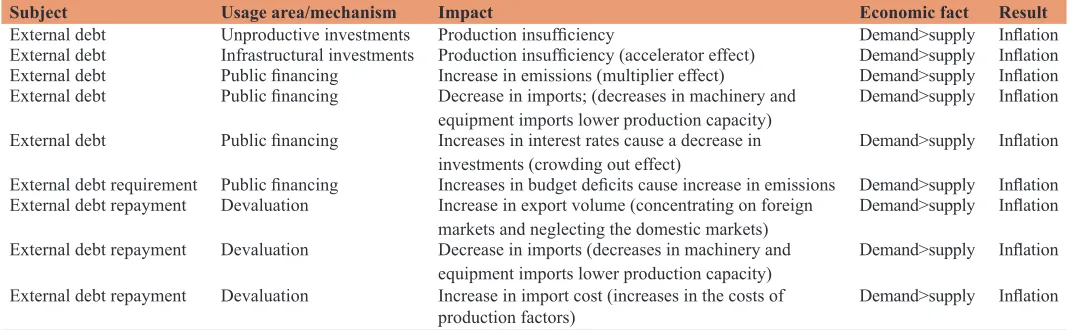
As can be seen from Table 1, external debt results in inflationary effects in many aspects. However, it should be noted that the main economic fact underlying this relationship is the insufficiency of supply to demand.
3. EXB AND INFLATION IN TURKEY FROM
2003 TO 2015
Quarterly total external debt stock of Turkey from 2003 to 2015 is available in Table 2.
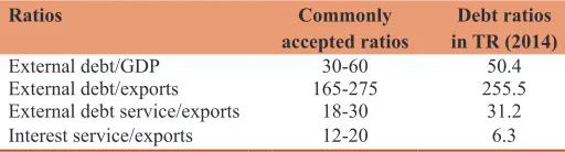
As can be seen in Table 2, the external debt stock of Turkey increased gradually between 2003 and 2015. The amount of debt eventuated as 130,931 million US Dollars in early 2003 reaching 405,223 million US Dollars in the midst of 2015. Many ratios are used to calculate the external indebtedness rate of a country. The commonly accepted external indebtedness ratios can be classified into four groups as shown in Table 3.
In accordance with the data for 2014, the following interpretations could be made by considering the commonly accepted external debt ratios of Turkey in Table 3:
• External debt/GDP in Turkey is 50.4% which remains within normal limits. Turkey, therefore, takes its place in the table of medium level indebted countries in terms of this ratio • External debt/exports in Turkey is 255.5% which is also between
the accepted limits. It shows that the export volume of Turkey allows it to cover a certain amount of its external debt stock • External debt service/exports in Turkey is 31.2%. This ratio
is above the upper limit. Although it is not in a very risky position, Turkey has a fragile capacity to render its principal and interest rate by its export revenues
• Interest service/export in Turkey is 6.3%. This is below even the lowest level of the commonly accepted ratio. This proves that the external debt interest can be paid easily through export gains.
As Karagöz (2007: 100) mentions, the World Bank takes two main measures into account with regard to borrowing. The first is “external debt/GDP” and the second “external debt service/ exports.” These two measures show the repayment capacity of a country. From a different point of view, since the first measure indicates revenue generating capacity and the second shows the foreign exchange-gaining possibility of an economy, they are significant for both internal and EXBs. While for Turkey the “external debt/GDP” lies between the commonly accepted rates, the rate of “external debt service/exports” was above the said limit as of end of 2014. The external debt service should, therefore, be tackled with care.
As shown in Table 4, starting from 2003 to 2015, there has, with minor exceptions, always been an upward tendency in inflation, in terms of CPI. This holds good for PPI too, as can be seen in Table 5.
Considering the inflationary process of Turkey from 2003 to 2015 in terms of both CPI and PPI, it may be asserted that there is a positive relationship between external debt and inflation. However, this requires to be tested. For this purpose a simple linear regression analysis has been made under the following title.
4. METHODOLOGY AND FINDINGS;
REGRESSION ANALYSIS FOR THE
EFFECTS OF EXTERNAL DEBTS ON
INFLATION IN TURKEY FROM 2003 TO 2015
Here, the effect of EXB on inflation rates in Turkey is measured through a simple linear regression analysis. In this context, both CPI and PPI are used. The aim is to confirm that EXB by Turkey had a positive effect on the inflation rate between 2003 and 2015. 50 observations of EXB, CPI, and PPI were used in the analysis. EXB data were collected from the Public Finance statistics of the Treasury of Turkey, while CPI and PPI data were taken from theTable 1: Interaction mechanism between external debt and inflation
Subject Usage area/mechanism Impact Economic fact Result
External debt Unproductive investments Production insufficiency Demand>supply Inflation
External debt Infrastructural investments Production insufficiency (accelerator effect) Demand>supply Inflation
External debt Public financing Increase in emissions (multiplier effect) Demand>supply Inflation
External debt Public financing Decrease in imports; (decreases in machinery and
equipment imports lower production capacity) Demand>supply Inflation External debt Public financing Increases in interest rates cause a decrease in
investments (crowding out effect) Demand>supply Inflation External debt requirement Public financing Increases in budget deficits cause increase in emissions Demand>supply Inflation
External debt repayment Devaluation Increase in export volume (concentrating on foreign
markets and neglecting the domestic markets) Demand>supply Inflation External debt repayment Devaluation Decrease in imports (decreases in machinery and
equipment imports lower production capacity) Demand>supply Inflation External debt repayment Devaluation Increase in import cost (increases in the costs of
inflation and price statistics of the Statistical Institute of Turkey. It should be noted that as there were only monthly data for CPI and PPI, the quarterly rates were calculated and used by the Author in the analysis. Monthly values are available in Appendix 1.
However, as Granger and Newbold (1974: 111-112) pointed out, since regression analysis with time series data may lead to spurious regression problems if the data are non-stationary, the levels of integration of the data set should be checked before starting the analysis. In this context, the autocorrelation, causality, and heteroscadasticity of the variables were examined. For these, linear unit root tests by Dickey-Fuller (Augmented Dickey-Fuller: ADF) and Phillips-Perron (PP) plus Granger Causality Tests were applied. Also heteroscadasticity of the variables was tested. The aim of such tests was to figure out whether regression results were unbiased and efficient. The tests were performed through the EViews 8 while the regression analyses were performed through the MS Excel.
4.1. Tests for the Variables of the Analysis
According to the Dickey-Fuller (ADF) Unit Root Test (1981) the presence/absence of unit root is very significant in figuring
out whether a time series is stationary. The series is appropriate for the analysis if it has a unit root and can be removed by the differencing method. Here the ‘‘τ (tau)’’ statistic of the Monte Carlo Study by Dickey and Fuller (1979) is used. If the absolute value of ‘‘τ (tau)’’ exceeds the absolute critical values by Dickey-Fuller or MacKinnon Dickey-Fuller, the assumption of stationarity of time series cannot be rejected. If “Ho: p=1” is rejected then the time series is stationary.
The Dickey-Fuller test assumes that error terms are statistically independent and have constant variance. Therefore, one should be sure that there is no correlation between error terms and they have constant variance (Altunöz, 2013: 187). Phillips and Perron (1988), broadened this assumption of Dickey-Fuller. They ignored the independence and homogenity assumptions of Dickey-Fuller and supposed weakly dependent and possibly heterogenously distributed data. Thus, it is clear that PP did not take into consideration the restrictions on the assumptions of error terms when developing Dickey-Fuller t-statistics.
According to the results in the Table 6, ADF-t statistical values for EXB, CPI, and PPI exceed Mackinnon’s (1991) critical value of 5% significance level. Therefore; EXB, CPI, and PPI variables are stationary according to first differences. All variables are stationary although they are at different significance levels. In other words, the variables used in this analysis do not contain unit roots and there is no contrariness for the predictions.
However, for the autocorrelation problem lag numbers are used.
As available in the Table 7, autocorrelation problem is solved when a lag length of 2 is used.
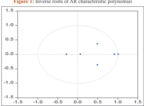
The polynomial can be assessed as an indicator of the stationarity of the model as well.
As can be seen in Figure 1, the position of inverse roots of the AR characteristic polynomial of the model also shows that there is no problem in terms of the stationarity of the Model. As none of the inverse roots are outside the unit encirclement, the established
Table 2: Quarterly external debt stock of Turkey from 2003 to 2015 (million USD)
Quarter Amount Quarter Amount Quarter Amount Quarter Amount
2003 Q1 130,931 2007 Q1 214,220 2011 Q1 301,994 2015 Q1 393,135
2003 Q2 135,040 2007 Q2 224,492 2011 Q2 313,683 2015 Q2 405,223
2003 Q3 138,722 2007 Q3 236,444 2011 Q3 312,123
2003 Q4 144,161 2007 Q4 250,012 2011 Q4 303,931
2004 Q1 144,800 2008 Q1 265,048 2012 Q1 316,747
2004 Q2 147,353 2008 Q2 287,156 2012 Q2 322,691
2004 Q3 153,105 2008 Q3 291,984 2012 Q3 327,496
2004 Q4 161,139 2008 Q4 280,957 2012 Q4 339,042
2005 Q1 160,322 2009 Q1 265,563 2013 Q1 352,109
2005 Q2 162,686 2009 Q2 268,180 2013 Q2 367,803
2005 Q3 166,472 2009 Q3 271,275 2013 Q3 373,499
2005 Q4 170,750 2009 Q4 268,963 2013 Q4 389,146
2006 Q1 185,545 2010 Q1 267,487 2014 Q1 388,244
2006 Q2 191,622 2010 Q2 265,741 2014 Q2 402,368
2006 Q3 197,246 2010 Q3 284,062 2014 Q3 397,781
2006 Q4 208,108 2010 Q4 292,057 2014 Q4 402,720
Source: Treasury of Turkey (2015), Public Finance Statistics. Retrieved on 15 October 2015 from the Treasury of Turkey Web site: http://www.treasury.gov.tr/en-US/ Stat-List?mid=738&cid=12&nm=684
Table 3: Commonly accepted external debt ratios and Turkey (%)
Ratios Commonly
accepted ratios in TR (2014)Debt ratios
External debt/GDP 30-60 50.4
External debt/exports 165-275 255.5 External debt service/exports 18-30 31.2 Interest service/exports 12-20 6.3
VAR system is stable and there are no different variances. Thus, the Model is stable in this context.
At this stage, the variables should be settled from outer to inner in the VAR analysis prediction. For this, the granger causality test that can
Table 4: Quarterly CPI in Turkey from 2003 to 2015 (%)
Quarter Rate Quarter Rate Quarter Rate Quarter Rate
2003 Q1 96.37 2007 Q1 136.64 2011 Q1 183.74 2015 Q1 252.64
2003 Q2 99.75 2007 Q2 139.68 2011 Q2 188.40 2015 Q2 259.92
2003 Q3 100.49 2007 Q3 139.17 2011 Q3 188.69
2003 Q4 103.39 2007 Q4 144.63 2011 Q4 198.95
2004 Q1 105.51 2008 Q1 148.68 2012 Q1 203.02
2004 Q2 107.15 2008 Q2 154.12 2012 Q2 206.14
2004 Q3 108.61 2008 Q3 155.38 2012 Q3 205.76
2004 Q4 113.13 2008 Q4 160.44 2012 Q4 212.42
2005 Q1 114.60 2009 Q1 161.12 2013 Q1 217.65
2005 Q2 116.38 2009 Q2 162.90 2013 Q2 220.52
2005 Q3 117.20 2009 Q3 163.67 2013 Q3 222.85
2005 Q4 121.75 2009 Q4 169.60 2013 Q4 228.30
2006 Q1 123.86 2010 Q1 176.09 2014 Q1 235.09
2006 Q2 127.56 2010 Q2 177.92 2014 Q2 241.25
2006 Q3 129.89 2010 Q3 177.39 2014 Q3 243.44
2006 Q4 133.71 2010 Q4 182.20 2014 Q4 248.30
Source: Statistical Institute of Turkey (2015-a), inflation and price. Retrieved on 15 October 2015 from the Statistical Institute of Turkey Web site: http://www.turkstat.gov.tr/UstMenu. do?metod=temelist. The quarterly rates were calculated by the monthly values of the Statistical Institute of Turkey. Monthly values are available in the Appendix 1, CPI: Consumer price
index
Table 5: Quarterly PPI in Turkey from 2003 to 2015 (%)
Quarter Rate Quarter Rate Quarter Rate Quarter Rate
2003 Q1 97.33 2007 Q1 136.39 2011 Q1 185.61 2015 Q1 239.35
2003 Q2 101.09 2007 Q2 139.11 2011 Q2 189.52 2015 Q2 247.45
2003 Q3 98.93 2007 Q3 140.55 2011 Q3 192.79
2003 Q4 100.80 2007 Q4 142.63 2011 Q4 200.56
2004 Q1 106.34 2008 Q1 147.81 2012 Q1 203.22
2004 Q2 110.86 2008 Q2 161.42 2012 Q2 203.51
2004 Q3 109.63 2008 Q3 161.88 2012 Q3 202.23
2004 Q4 115.48 2008 Q4 158.61 2012 Q4 206.32
2005 Q1 115.63 2009 Q1 156.52 2013 Q1 207.30
2005 Q2 119.50 2009 Q2 158.89 2013 Q2 209.67
2005 Q3 121.38 2009 Q3 159.50 2013 Q3 215.19
2005 Q4 122.25 2009 Q4 162.58 2013 Q4 219.67
2006 Q1 123.83 2010 Q1 167.85 2014 Q1 231.78
2006 Q2 130.63 2010 Q2 173.33 2014 Q2 233.41
2006 Q3 135.66 2010 Q3 173.42 2014 Q3 236.12
2006 Q4 135.41 2010 Q4 177.18 2014 Q4 237.82
Source: Statistical Institute of Turkey (2015-a), inflation and price. Retrieved on 15 October 2015 from the Statistical Institute of Turkey Web site: http://www.turkstat.gov.tr/UstMenu. do?metod=temelist., The quarterly rates were calculated by monthly values of the Statistical Institute of Turkey. Monthly values are available in Appendix II, PPI: Producer price index
Table 6: Linear unit root test results
Variable ADF statistics (level) PP statistics (level)
EXB –2.922 –2.922
CPI –2.926 –2.922
PPI –2.928 –2.928
Variables on first differences (constant and inconstant)
EXB –3.506 –3.506
CPI –3.518 –3.506
PPI –3.510 –3.506
MacKinnon 5% critical value: Level (constant): –2.9; First difference (constant
and inconstant): –3.5, Lags were determined in accordance with the Schwarz
Information Criterion, Tests were performed through EViews 8, EXB: External borrowing, PPI: Producer price index, CPI: Consumer price index, PP: Phillips-Perron,
ADF: Augmented Dickey-Fuller
Table 7: Lags for autocorrelation problem
Lags LM-statistics Probability
1 5.960573 0.7439
2 3.529407 0.9396
3 6.454472 0.6937
4 5.482571 0.7904
5 8.745679 0.4611
6 3.569288 0.9374
be done through VAR analysis with positive significance test results following the determination of appropriate lag numbers is applied.
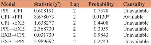
As can be seen in the Table 8, there is a causality between CPI→PPI at 5% significance level. However, there is no relation between other variables (PPI→CPI, CPI→EXB, PPI→EXB, EXB→CPI, EXB→PPI).
The results of the white heteroscedasticity test applied to determine whether the variance of error terms is constant for whole sample, are shown Table 9.
It is seen in the Table 9 that the variance of time error term is constant for all observations. That is, there is no variance problem (p=0.8458>5%). In this case, “Ho” is accepted and an inconstant variance problem is not available (null hypothesis: No heteroscedasticity).
4.2. Model 1: Simple Linear Regression Analysis for EXB and CPI
This model includes 50 observations for the period 2003-2015. The regression analysis summary outputs are available in the Appendix 3. Variables of the model are as follows:
Dependent variable (Y) : CPI Independent variable (X) : EXB
As the relationship between the variables of the model is positive, a linear regression analysis is applied.
Y = b0 b1X + Ɛ
Inflation (CPI) = b0 + b1 (EXB) + Ɛ
Y = 21.75424209+ 0.000546646 X + Ɛ
Standard Error : (4.083334534) (1.46847E-05)
tstatistics : (5.327567924) (37.22559373)
R2 = 0.966521239
Adjusted R2 = 0.965823765
Assessments of the results are as follows:
• b0: 21.75; even if there is no EXB, there will be a CPI of 21.75. • b1: 0.00055; 1 unit EXB causes a 0.00055 unit increase in CPI.
Now, we try to figure out if the model is significant. For this purpose F-test shall be applied. Here are the hypotheses:
• H0: b=0 (It is not significant that the model best fits the population from which the data were sampled; that is Model is not significant).
• H1: b≠0 (It is significant that the model best fits the population from which the data were sampled; that is Model is significant).
If F value > critical value of F distribution, then the null hypothesis is rejected. As F value=1385.745 > critical value of F distribution=1.61, we reject the null hypothesis. That is the Model is significant which means that EXB increases CPI.
It is time to check whether the coefficients are statistically significant. For this purpose, T-test shall be applied and, in this context, the values of tstatistics and ttable shall be compared. Here are the hypotheses:
• H0: b=0 (a unit change in X does not make any change in Y; that is, there is no correlation between these two variables). • H1: b≠0 (a unit change in X makes a significant change in Y;
that is, there is a correlation between these two variables).
If the value of a is 0.05, then ttable is 1.68. In this case if tstatistics > ttable, it means that the coefficients are statistically significant. As tstatistics for b1 =37.23 > ttable for b1=1.68, coefficient b1 is statistically significant which means that there is a positive correlation between EXB and CPI.
Another measure to interpret the model is the coefficients of determination:
R2 = 0.966
Adjusted R2 = 0.966
Values of coefficients of determination show the strength of the relationship between the dependent and independent variables. Both R2 and Adjusted R2 are high (97%) which means that the model is reliable. In a word, these coefficients show that the 97% increase in the CPI is explained by EXB in Turkey for the period 2003-2015.
4.3. Model 2: Simple Linear Regression Analysis for EXB and PPI
This model also includes 50 observations for the period 2003-2015. The regression analysis summary outputs are available in Appendix IV. Variables of the model are as follows:
Dependent variable (Y) : PPI Independent variable (X) : EXB
As the relationship between the variables of the model is positive, a linear regression analysis is applied here too.
Y = b0 + b1X + Ɛ
Inflation (PPI) = b0 + b1 (EXB) + Ɛ
Y = 30.01116 + 0.000508 X + Ɛ
Standard Error : (3.559362) + (1.28E-05)
tstatistics : (8.431611) (39.66731)
R2 = 0.970398
Adjusted R2 = 0.969781
Table 8: Granger causality test results
Model Statistic (χ2) Lag Probability Causality
PPI→CPI 0.608191 2 0.7378 Unavailable
CPI→PPI 8.678073 2 0.0130* Available
CPI→EXB 1.638277 2 0.4408 Unavailable
PPI→EXB 2.368730 2 0.3059 Unavailable
EXB→CPI 0.031739 2 0.9843 Unavailable
EXB→PPI 2.989692 2 0.2243 Unavailable
Lags were determined in accordance with the Akaike Criterion, *shows 5% significance level
Table 9: White heteroscedasticity test results
Chi‑squares df Probability
Assessments of the results are as follows:
• b0: 30.01; even if there is no EXB there will be a PPI of 30.01. • b1: 0.00051; 1 unit EXB causes a 0.00051 unit increase in PPI.
For showing the significance of the Model we apply F-test. As F value=1,573.496 > critical value of F distribution=1.61, the null hypothesis is rejected. That is the Model is significant which means that EXB increases PPI.
As another component of model assessment for checking whether the coefficients are statistically significant, T-test shall be applied.
As tstatistics for b1 =39.67 > ttable for b1=1.68, coefficient b1 is statistically significant. That is, EXB increases PPI.
The interpretation of determination coefficients is given below:
R2 = 0.970
Adjusted R2 = 0.970
In this model, both R2 and Adjusted R2 are high (97%) which means that the model is reliable. That is, the 97% increase in PPI is explained by EXB in Turkey in the said period.
5. CONCLUSION
Different views on borrowing can be found. As quoted by Tuna (2014), while David Ricardo defined public borrowing as “an awful scourge invented at any time to torment the people,” nearly 100 years later, Lorenz von Stein, a Finance Officer in Germany, opposing this idea said that “a debtless country either does fewer things for its future or demands many things from the moment.” Considering these approaches it is clear that on the one hand, while inflation as a result of EXB becomes a means to torment the people, on the other hand it is also the result of investment, public financing, growth etc.
In this paper, both effects have been examined for Turkey. Firstly, the simple linear regression analyses confirm that the use of EXB has resulted in increased inflation rates. These analyses show that both the CPI and the PPI have been affected by the EXB in Turkey from 2003 to 2015. That is, EXB has increased both CPI and PPI through various mechanisms. Secondly, it is obvious that EXB has had some positive results on some economic aggregates such as investments, the public budget and growth. However, these have also had indirect effects on inflation due to some negative aspects of Turkey’s economy. One of which may, be the lack of well organised financial markets in addition to other shortfalls. The main factors for foreign debt being a cause of inflation in the economy of Turkey may be a misuse of these sources for unproductive investments, huge infrastructural investments, public deficits, and an imbalance of payments.
Ulusoy and Küçükkale (1996: 24), while considering that external debts used for infrastructural investments cause inflation, say that if external debts were used to finance income-generating investments (especially for gaining foreign exchange), the debts
could be repaid and factor endowments increased in favour of capital. Thus, it would be possible to provide growth without accelerating the inflationary process.
Duran (1996: 442) says that direct income-generating public investment expenditures could be financed by EXB as they provide direct revenue for the servicing of principal and interest. However, maturity of the debt should be equal to the terms of return on investment. The most significant component of such financing is the difference between the real interest rate and the return on investment ratio. He adds that it is advantageous to finance investment by EXB provided the real interest rate is either negative or less than the return on investment ratio. In any case, taxation would be preferable to long term, unmeasurable and indirect income-generating public investments.
Evgin (2000: 13) emphasises that while there have been brilliant successes in decreasing inflation in several countries, increases in external debt may frustrate these results and that strong budget discipline together with monetary stability measures are the sole solution for success in this respect. An expansionary monetary and budgeting policy may result in economic crises as happened in Germany in the 1920s and in the USA in the 1930s. She asserts that continuous economic growth is possible only through implementation of a stable monetary policy and strong budget discipline. Only these policies can decrease interest rates by dashing inflationary expectations and lowering public debt burden to a bearable level.
Karagöz (2007: 109) asserts that covering a deficit in the balance of payments rather than dealing with the shortfall in internal savings has been the main reason for the need for EXB in Turkey. In his study he states that by providing balance of payments, new financial resources should be generated and current debts be repaid before further debts are incurred. For this purpose, while export revenues are increased, import expenditures should be decreased. Moreover, tourism revenues need to be increased and direct foreign investments fostered. Furthermore, internal borrowing with its positive effect on internal savings and with less foreign exchange risk, may be preferable to EXB. Sugözü and Yiyit (2010: 371), on the other hand, in agreement with Classical Economists say that borrowing should be the last financial choice made and only then under obligatory circumstances such as the need for financing huge amounts of investment due, for example, to natural disasters and war.
6. ACKNOWLEDGMENT
The Author thanks to the anonymous referees for their comments. His special thanks go to İbrahim Akkaş and Basri Çınar, Research Assistants, Economics, Mardin Artuklu University for their suggestions
REFERENCES
Adıyaman, A.T. (2006), Dış Borçlarımız ve Ekonomik Etkileri. Sayıştay
Dergisi, 62, 21-45.
Altunöz, U. (2013), Türkiye’de enflasyon, büyüme ve finansal derinleşme ilişkisinin ampirik analizi. Kahramanmaraş Sütçü İmam Üniversitesi İİİBF Dergisi, 3(2), 175-195.
Burguet, R., Fernandez-Ruiz, J. (1998), Growth through taxes or
borrowing? A model of development traps with public capital.
European Journal of Political Economy, 14, 327-344.
Cardoso, E., Fishlow, A. (1990), External debt, budget deficits, and inflation. In: Sachs, J.D., editor. Country Debt and Economic Performance, Vol. 2: The Country Studies - Argentina, Bolivia, Brazil, Mexico. Chicago: University of Chicago Press. p318-334. Available from: http://www.nber.org/chapters/c8948.
Central Bank of Turkey. (2015a), Balance of Payment Statistics. Central Bank of Turkey. Available from: http://www.tcmb.gov.tr/wps/wcm/ connect/TCMB+EN/TCMB+EN/Main+Menu/STATISTICS/Balan ce+of+Payments+and+Related+Statistics/Balance+of+Payments+ Statisticss/. [Last retrieved on 2015 Oct 16].
Central Bank of Turkey. (2015b), Outstanding Loans Received from Abroad by Private Sector; Definitions and Explanations. The Central Bank of Turkey. Available from: http://www.tcmb.gov.tr/wps/ wcm/connect/bc4ba7ca-2241-46ae-8c6c-589c9aa1faaa/definition. pdf?MOD=AJPERES. [Last retrieved on 2015 Oct 16].
Chaudhary, M.A., Anjum, S.W. (1996), Macroeconomic policies and management of debt, deficit, and inflation in Pakistan. The Pakistan Development Review, 35(4), 773-786.
Demir, M., Çevik, S., Beşer, M.K. (2005), Kamu kesimi finansman açiklarinin ekonomik etkileri: Türkiye üzerine bir inceleme. Marmara Üniversitesi İİBF Dergisi 20(1), 247-267.
Demir, M., Sever, E. (2009), Kamu Açıkları ve Borçlanma İlişkisi: Türkiye, Azerbaycan, Kazakistan ve Kırgızistan Üzerine Bir Uygulama, Sosyo Ekonomi, Ocak-Haziran. p8-26.
Dickey, D.A., Fuller, W.A. (1979), Distribution of the estimators for
autoregressive time series with a unit root. Journal of the American Statistical Association, 74(366), 427-431.
Dickey, D.A., Fuller, W.A. (1981), Likelihood ratio statistics for
autoregressive time series with a unit root, Econometrica, 49(4), 1057-1072.
Duran, M. (1996), Kamu Finansman Açıklarının Optimal Finansmanı. In: Kamu Kesimi Finansman Açıkları: X. Maliye Sempozyumu, Mayıs 1994, Antalya, İstanbul Üniversitesi Basımevi. p435-453.
Evgin, T. (2000). Dünden Bugüne Dış Borçlarımız. Hazine Müsteşarlığı, Ekonomik Araştırmalar Genel Müdürlüğü, Ankara, Haziran. Granger, C.W.J., Newbold, P. (1974), Spurious Regressions in
Econometrics. Journal of Econometrics, 2, 111-120.
Karakaplan, M.U. (2009), The conditional effects of external debt on inflation. Selçuk Üniversitesi İİBF Sosyal ve Ekonomik Araştırmalar Dergisi, 11(17), 203-217.
Karagöz, K. (2007), Türkiye’de diş borçlanmanin nedenleri; ekonometrik bir değerlendirme. Sayıştay Dergisi, 66-67, 99-110.
Kim, Y.J., Zhang, J. (2012), Decentralized borrowing and centralized
default. Journal of International Economics, 88, 121-133.
Lessard R.D. (1986), International Financing for Developing Countries. World Bank Staff Working Paper, No: 793, Series on International Capital and Economic Development. Washington, DC.
Mackinnon, J.G. (1991). Criticial values for cointegration tests. In: Engle, R.F., Granger, C.W.J., editors. Long-Run Economic Relationship: Readings in Cointegration, New York: Oxford University Press. Makin, A.J., Narayan, P.K. (2013), Has international borrowing or
lending driven Australia’s net capital inflow? International Review
of Economics and Finance, 27, 134-143.
Phillips, P.C.B., Perron, P. (1988), Testing for a unit root in time series
regression. Biometrika, 75(2), 335-346.
Prokop, J., Baranowska-Prokop, E. (2012), The efficiency of foreign borrowing: The case of Poland. In: International Conference on Applied Economics (ICOAE). Procedia Economics and Finance, 1, 321-329, Sugözü, İ.H., Yiyit, M. (2010), Borçlanmanın enflasyona etkisi üzerine
teorik yaklaşimlarin temel özellikleri. Maliye Dergisi, 158, 365-373. Statistical Institute of Turkey (2015a), Inflation and Price. Statistical
Institute of Turkey. Available from: http://www.turkstat.gov.tr/ UstMenu.do?metod=temelist. [Last retrieved on 2015 Oct 15]. Statistical Institute of Turkey (2015b), National Accounts. Statistical
Institute of Turkey. Available from: http://www.turkstat.gov.tr/ UstMenu.do?metod=temelist. [Last retrieved on 2015 Oct 15]. Treasury of Turkey (2015), Public Finance Statistics. Treasury of
Turkey. Available from: http://www.treasury.gov.tr/en-US/Stat-List?mid=738&cid=12&nm=684. [Last retrieved on 2015 Oct 15]. Tuna, Y. (2014), Türkiye’de Kamu Kesimi Açıkları. Available from: http://
www.ekodialog.com/Makaleler/turkiyede_kamu_kesimi_aciklari.
html. [Last retrieved on 2014 Jul 25].
Ulusoy, A., Küçükkale, Y. (1996), Türkiye’de borçlarin iktisadî büyüme ve enflasyon üzerine etkisi. Granger Nedensellik Testi Ekonomik Yaklaşım, 7(21), 15-25.
Wang, F. (2009), The effects of foreign borrowing policies on economic growth: Success or failure? Journal of Economic Policy Reform,
12(4), 273-284.
Appendix 1: Monthly CPI in Turkey from 2003 to 2015 (%)
Months 2003 2004 2005 2006 2007 2008 2009 2010 2011 2012 2013 2014 2015
January 94.77 104.81 114.49 123.57 135.84 146.94 160.90 174.07 182.60 201.98 216.74 233.54 250.45
February 96.23 105.35 114.51 123.84 136.42 148.84 160.35 176.59 183.93 203.12 217.39 234.54 252.24 March 98.12 106.36 114.81 124.18 137.67 150.27 162.12 177.62 184.70 203.96 218.83 237.18 255.23 April 99.09 106.89 115.63 125.84 139.33 152.79 162.15 178.68 186.30 207.05 219.75 240.37 259.39
May 100.04 107.35 116.69 128.20 140.03 155.07 163.19 178.04 190.81 206.61 220.07 241.32 260.85
June 100.12 107.21 116.81 128.63 139.69 154.51 163.37 177.04 188.08 204.76 221.75 242.07 259.51
July 99.93 107.72 116.14 129.72 138.67 155.40 163.78 176.19 187.31 204.29 222.44 243.17 August 100.09 108.54 117.13 129.15 138.70 155.02 163.29 176.90 188.67 205.43 222.21 243.40
September 101.44 109.57 118.33 130.81 140.13 155.72 163.93 179.07 190.09 207.55 223.91 243.74 October 102.38 112.03 120.45 132.47 142.67 159.77 167.88 182.35 196.31 211.62 227.94 248.37 November 103.68 113.50 122.14 134.18 145.45 161.10 170.01 182.40 199.70 212.42 227.96 248.82 December 104.12 113.86 122.65 134.49 145.77 160.44 170.91 181.85 200.85 213.23 229.01 247.72
Source: Statistical Institute of Turkey (2015-a). Inflation and Price, Retrieved on 15 October 2015 from the Statistical Institute of Turkey Web site: http://www.turkstat.gov.tr/UstMenu. do?metod=temelist
Appendix 2: Monthly PPI in Turkey from 2003 to 2015 (%)
Months 2003 2004 2005 2006 2007 2008 2009 2010 2011 2012 2013 2014 2015
January 94.32 104.46 114.83 123.51 135.09 143.80 155.16 164.94 182.75 203.10 206.91 229.10 236.61 February 97.28 106.17 114.81 123.83 136.37 147.48 156.97 167.68 185.90 202.91 206.65 232.27 239.46
March 100.40 108.40 117.25 124.14 137.70 152.16 157.43 170.94 188.17 203.64 208.33 233.98 241.97
April 102.17 111.27 119.62 126.54 138.80 159.00 158.45 174.96 189.32 203.81 207.27 234.18 245.42 May 101.53 111.24 119.23 130.05 139.34 162.37 158.37 172.95 189.61 204.89 209.34 232.96 248.15 June 99.58 110.06 119.64 135.28 139.19 162.90 159.86 172.08 189.62 201.83 212.39 233.09 248.78 July 99.04 108.39 119.33 136.45 139.28 164.93 158.74 171.81 189.57 201.20 214.50 234.79
August 98.85 109.25 121.40 135.43 140.47 161.07 159.40 173.79 192.91 201.71 214.59 235.78 September 98.90 111.26 123.40 135.11 141.90 159.63 160.38 174.67 195.89 203.79 216.48 237.79
October 99.46 114.85 124.22 135.73 141.71 160.54 160.84 176.78 199.03 204.15 217.97 239.97
November 101.15 115.72 121.40 135.33 142.98 160.49 162.92 176.23 200.32 207.54 219.31 237.65 December 101.78 115.87 121.14 135.16 143.19 154.80 163.98 178.54 202.33 207.29 221.74 235.84
Source: Statistical Institute of Turkey (2015-a). Inflation and Price, Retrieved on 15 October 2015 from the Statistical Institute of Turkey Web site: http://www.turkstat.gov.tr/UstMenu. do?metod=temelist
Appendix 3: Regression analysis summary outputs for external borrowing and CPI in Turkey from 2003 to 2015
Summary output
Regression statistics
Multiple R 0.983118121
R square 0.966521239
Adjusted R square 0.965823765
Standard error 8.803423529
Observations 50
ANOVA
df SS MS F Significance F
Regression 1 107395.5926 107395.5926 1385.744828 4.57738E-37
Residual 48 3720.01276 77.50026583
Total 49 111115.6053
Coefficients Standard error t stat P value Lower 95% Upper 95%
Intercept 21.75424209 4.083334534 5.327567924 2.61965E-06 13.54414775 29.96433643
X variable (Ext. Debt) 0.000546646 1.46847E-05 37.22559373 4.57738E-37 0.000517121 0.000576172
Appendix 4: regression analysis summary outputs for external borrowing and PPI in Turkey from 2003 to 2015
Summary output
Regression statistics
Multiple R 0.985088
R Square 0.970398
Adjusted R square 0.969781
Standard error 7.67377 Observations 50
ANOVA
df SS MS F Significance F
Regression 1 92658.05 92658.05 1573.496 2.38E-38
Residual 48 2826.564 58.88675
Total 49 95484.61
Coefficients Standard error t stat P value Lower 95% Upper 95%