RESEARCH
Combining self-organizing maps and biplot
analysis to preselect maize phenotypic
components based on UAV high-throughput
phenotyping platform
Liang Han
1,2,4†, Guijun Yang
1*†, Huayang Dai
4, Hao Yang
1,3, Bo Xu
1, Heli Li
3, Huiling Long
1,3, Zhenhai Li
3,
Xiaodong Yang
1,3and Chunjiang Zhao
1,3*Abstract
Background: With environmental deterioration, natural resource scarcity, and rapid population growth, mankind is facing severe global food security problems. To meet future needs, it is necessary to accelerate progress in breeding for new varieties with high yield and strong resistance. However, the traditional phenotypic screening methods have some disadvantages, such as destructive, inefficient, low-dimensional, labor-intensive and cumbersome, which seri-ously hinder the development of field breeding. Breeders urgently need a high-throughput technique for acquiring and evaluating phenotypic data that can efficiently screen out excellent phenotypic traits from large-scale genotype populations.
Results: In the present study, we used an unmanned aerial vehicle (UAV) high-throughput phenotyping (HTP) platform to collect RGB and multispectral images for a breeding program and acquired multiple phenotypic compo-nents (or traits), such as plant height, normalized difference vegetation index, biomass accumulation, plant-height growth rate, lodging, and leaf color. By implementing self-organizing maps and principal components analysis biplots to establish phenotypic map and similarity, we proposed an UAV-assisted HTP framework for preselecting maize (Zee mays L.) phenotypic components (or traits).
Conclusions: This framework gives breeders additional information to allow them to quickly identify and preselect plants that have genotypes conferring desirable phenotypic components out of thousands of field plots. The present study also demonstrates that remote sensing is a powerful tool with which to acquire abundant phenotypic compo-nents. By using these rich phenotypic components, breeders should be able to more effectively identify and select superior genotypes.
Keywords: SOM, Biplot, UAV, Maize, High-throughput phenotyping
© The Author(s) 2019. This article is distributed under the terms of the Creative Commons Attribution 4.0 International License (http://creat iveco mmons .org/licen ses/by/4.0/), which permits unrestricted use, distribution, and reproduction in any medium, provided you give appropriate credit to the original author(s) and the source, provide a link to the Creative Commons license, and indicate if changes were made. The Creative Commons Public Domain Dedication waiver (http://creat iveco mmons .org/ publi cdoma in/zero/1.0/) applies to the data made available in this article, unless otherwise stated.
Open Access
*Correspondence: [email protected]; [email protected] †Liang Han and Guijun Yang contributed equally to this work and should be considered co-first author
1 Key Laboratory of Quantitative Remote Sensing in Agriculture of Ministry of Agriculture, Beijing Research Center for Information Technology in Agriculture, Beijing 100097, China
effective measures for plant breeders and geneticist to alleviate the current situation. In the last two decades, crop sequencing technology has developed rapidly, allowing the whole genome to be sequenced rapidly at low cost. However, because of the lack of assistant phe-notypic knowledge, methods for rapid identification of desirable traits have advanced little [4, 5]. With increas-ing demand for rapid phenotypincreas-ing of large numbers of lines and to accelerate progress in breeding for novel traits, phenotyping is often considered the bottleneck of crop breeding [6].
Recent advance in high-throughput phenotyping (HTP) technologies has provided a positive response to narrow the gap between the wealth of genomic data with pheno-typic data [7]. HTP technologies allow large numbers of plants to be measured in a non-destructive manner with accuracy and precision. Initially, high-throughput phe-notyping was applied in controlled environments, such as greenhouses and growth chambers, to collect phe-notypic data from model organisms [8]. This is indoor shoot-based phenotyping that have an advantage in char-acterizing individual plants grown in pots, and not lim-ited by overlapping canopies and variable environmental conditions due to soil, temperature, water etc. However, the main concern for many breeders is that the complex traits obtained by using HTP technologies in controlled environments may not be fully replicated in the field, so phenotyping in field conditions remains a bottleneck that hinders advances in breeding [5, 6, 9].
With continuous advances in proximal sensing, field-based HTP has become widespread in the breeding programs. Recently, several field-based HTP platforms were developed to measure phenotypic traits, including ground-based HTP platforms [10–12] and aerial-based HTP platforms [13–15]. Ground-based HTP platforms consisting of modified vehicles have the advantages of high resolution, flexible design, and large payload, but have limitations in the portability and scale at which they can be used [16]. Compared to ground-based HTP plat-forms, aerial-based HTP platforms enable the rapid eval-uation of the populations consisting of thousands to tens of thousands of plots and the synchronized measure-ments of multiple traits in an efficient manner, overcom-ing some limitations associated with the ground-based
typing techniques are time-consuming, labor intensive and impractical for large-scale operations [20]. Despite the advantages of satellite remote sensing in large-scale observation, it remains some limitations, such as low resolution, long revisit period and high susceptibility to water vapor [21]. In conclusion, compared with other technologies, UAV-HTP offers excellent opportunities for rapid and non-destructive extraction of crop pheno-typic information in the field.
Currently, several structural and physiological agro-nomic traits suitable for HTP have been proposed for use in breeding programs, including but not limited to the normalized difference vegetation index (NDVI) [11, 22, 23], biomass accumulation [21, 24], plant height [25, 26], plant-height growth rate [15, 27, 28], lodging [29, 30], leaf color [24, 31], and yield [32–34]. Previous research has demonstrated that measurements provided by HTP plat-forms are highly correlated with manual reference meas-urements [26, 34, 35]. By using HTP technologies capable of collecting phenotypic data at multiple time points or throughout the season, researchers can better under-stand how traits develop, allowing better optimization of genotypes through selection in breeding programs [36].
A preliminary approach with easily measurable phe-notypic traits provides a chance to select genotypes [37]. Cluster and correlation analyses seem to be a promising approach for identifying potential associations between phenotype and genotype [38, 39], which clarifies gene co-expression and phenotypic similarity. Self-organiz-ing maps (SOMs) are a type of artificial neural network invented by Kohonen [40] that are trained by using unsu-pervised learning to project high-dimensional, complex data onto a two-dimensional grid. This reduces dimen-sionality and enhances the visualization of clustering [41, 42]. A principal components analysis (PCA) biplot high-lights the extent to which the objects in rows (samples) differ from the objects in columns (features) [43]. In this context, a PCA biplot shows the largest patterns in the data in terms of how the phenotypic components differ in different genotypes.
(or traits). The specific objectives for this study were (i) to propose an UAV-assisted HTP framework to establish phenotypic maps and similarities, (ii) to identify selection strategies for different breeding targets or multiple phe-notypic components, and (iii) to assess the potential for using UAV field-based HTP platforms for selection deci-sions in a large breeding program.
Methods
Field trials
Field breeding trials included a natural population and a doubled-haploid population (i.e., 800 maize plots). The natural population assessed in this study consisted of 482 maize plots divided into three subpopulations based on differences in genetic background: Mixed, temper-ate (TEM), and tropical or subtropical (TST). Of the 482 plots, 106 were from the mixed subpopulation, 162 were from the TEM subpopulation, and 214 were from the TST subpopulation.
The field trials were conducted at the research sta-tion of Xiao Tangshan Nasta-tional Precision Agriculture Research Center of China, Changping District of Beijing City (115°50′17″–116°29′49″E, 40°20′18″–40°23′13″N). The study area is in a warm temperate zone with a semi-humid continental monsoon climate. The annual average temperature is 11.8 °C, and the annual average precipi-tation is 550.3 mm. Eight hundred plots were arranged across a field measuring approximately 30 m by 196 m, with a spacing of 0.8 m between plots. Each plot con-sisted of three 2.4-m-long rows, each containing approxi-mately 27 plants spaced 25 cm apart. All plots were planted by using a seeder on May 15, 2017.
HTP platform and data acquisition
The two cameras used in this study were mounted on an UAV HTP platform (DJI Spreading Wings S1000, SZ DJI Technology Co., Shenzhen, China). The first camera was a Sony digital RGB high-resolution camera (DSC-QX100, 5472 × 3648 pixels, Sony Electronics, Inc., Tokyo, Japan) with the ISO and shutter speed set at 160 and 1/2000, respectively. The second camera was a Parrot Sequoia multispectral camera (1280 × 960 pixels, MicaSense Inc., Seattle, USA) that combines four monochrome sensors (green: 550 nm, red: 660 nm, red-edge: 735 nm, near-infrared: 790 nm) and can simultaneously capture four different band images with a 10 nm bandwidth (half maximum bandwidth) for the red-edge band and a 40 nm bandwidth for the green, red, and near-infrared bands. A sunshine sensor was used with the Sequoia sensors to minimize errors caused by variations in ambient light during acquisition (Fig. 1a).
Flight paths were designed by using the DJI ground sta-tion (SZ DJI Technology Co., Shenzhen, China) to ensure
80% forward overlap and 75% side overlap, yielding six strips. To build the digital elevation model (DEM), the above-ground-level (AGL) parameter for the first flight was set to 40 m, yielding a ground-sampling distance of 0.72 cm. The AGL parameter for four other flights was set to 60 m, yielding a ground-sampling distance of approxi-mately 1.33 cm. The radiometric calibration images were captured on the ground before and after each flight by using a calibrated reflectance panel (MicaSense Inc., Seattle, USA). Prior to the first flight, 16 ground con-trol point (GCP) markers were arranged evenly over the experimental site and were measured by using a differen-tial global positioning system (DGPS, South Surveying & Mapping Instrument Co., Ltd., Guangzhou, China) with millimeter accuracy.
Images were acquired five times over the period span-ning vegetative to reproductive growth (Fig. 1b). Table 1 details the flight conditions. The leaf collar method of Ritchie [44] was used for staging maize plant growth. Due to differences in genotype, heterogeneity appears in the growth and development at the plot scale. Therefore, the growth stage in Table 1 was determined by using the 50% majority rule.
Plant sampling and measurements
A total of 72 plots served as sampling plots for destruc-tive biomass measurements and plant-height measure-ments. Because of the consumption caused by destructive sampling, another 72 plots were selected for the meas-urement on August 3, 2017 (Fig. 1c). Three plants were selected at random from the middle of the sampling plots to measure plant height and fresh biomass. Plant height was manually measured by using a telescopic leveling rod. The mean height of three plants was used as plant height at the plot scale for the ground truth. The three selected plants were then used for destructive biomass sampling. The fresh biomass was sealed in plastic bags and weighed on the same day. By calculating the actual number of plants per sampling plot, the mass was rescaled to kg/m2.
We visually determined the color of the positive leaves at the plot scale and recorded the results. From July 1 to 10, 2017, lodging occurred in some plots due to frequent strong winds and rainfall. A field investigation was done for 800 plots and the results for were recorded for root lodging, stem breaking, and stem lodging. Table 2 gives the dates for sampling and measurements.
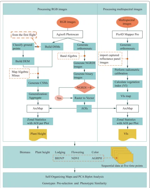
Image processing and data extraction
(DSMs) of each flight with the GCPs to optimize the camera position and ensure precise alignment [45]. A workflow (Han et al. 2018) was applied to create an area of interest for each plot by using the orthomosaics and to
build the DEM by using the DSMs. Multispectral images were processed with Pix4D Mapper Pro software (version 4.0, PIX4D, Lausanne, Switzerland). Pix4D Mapper Pro has advantages in radiometric calibration and vegetation index calculation and offers some important process-ing steps similar to Agisoft Photoscan, such as align-ing photos, importalign-ing GCPs and geographic references, building dense point clouds, and generating DSM and orthomosaics. Radiometric calibration was done by using the Pix4D Mapper Pro software with radiometric cali-bration images with known reflectance values provided by MicaSense. NDVI (or other vegetation indices) maps were then produced by using the index calculator.
Crop surface models (CSMs), which are widely used to extract crop height, were obtained by subtracting Fig. 1 Schematic diagram of trial design and field layout
Table 1 Flight conditions for acquiring images over period spanning vegetative to reproductive growth
a Days after sowing
Flight Date DASa AGL Growth stage
1 2017-06-08 24 40 V4
2 2017-06-29 45 60 V10
3 2017-07-11 57 60 V14
4 2017-07-28 78 60 VT
the DEM from the DSMs. By using the areas of inter-est, a workflow [21] was applied to extract phenotypic data such as plant height and NDVI for each plot in the field from CSM and NDVI maps. Figure 2 illustrates the complete preprocessing chain.
After transforming a RGB image into HSL (i.e., hue, saturation and lightness) color space by using ENVI soft-ware (version 4.5, Esri Inc., Redlands, USA) and com-bining with field-sampled data, we used the hue value in HSL color space to cluster the population and classi-fied the population into three leaf colors. Flowering was defined as a dichotomous variable that distinguishes whether flowering occurs at the fourth time point, as judged by visual observation of an orthomosaic. Average growth rate of plant height (AGRPH) is the increment in plant height per day between two adjacent time points [15]. Fresh biomass and BIOVP (a volume metric to esti-mate crop biomass within certain spatial ranges) were calculated following Han [21]. The identification of maize lodging was implemented following Han [29].
Self‑organizing map and hierarchical cluster analysis
Selective breeding requires analysis of the relationships between multiple phenotypic traits and focuses on geno-types that are differentially expressed and co-expressed under the same environmental conditions. Differential expression can be accomplished using statistically sig-nificant difference test, while co-expressed genotypes require cluster analysis to examine the relationship between individuals or groups at the multiple-traits level. To explore co-expressed genotypes and identify underly-ing agronomic groups with similar phenotypic compo-nents, we performed two-step clustering to isolate 482 samples with nine dimensions that we standardized to values by using the mean and standard deviation. Two-step clustering was done for a pre-clustering by using the self-organizing map (SOM) method, which generates a simplified representation of the original data set and converts nonlinear statistical relationships between high-dimensional data into simple geometric relationships between points on a two-dimensional map [46]. The pre-clusters were then subjected to agglomerative hierar-chical clustering (AHC), which projects similar samples
onto the same neuron. Finally, AHC analysis revealed the neighboring neurons of the topological map belonging to the same final cluster. A tree diagram was used to illus-trate the arrangement of the clusters produced by AHC and to understand and identify clusters.
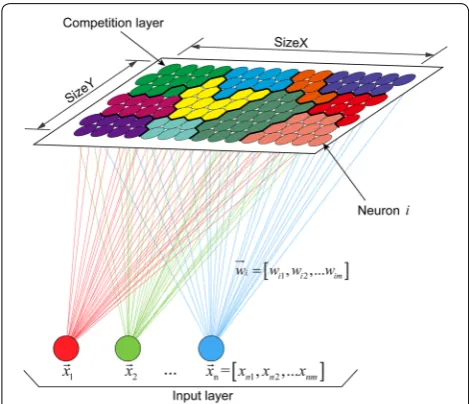
As shown in Fig. 3, the basic structure of the SOM net-work consists of an input layer and a competition layer. For mixed data in the input layer, an extra layer is cre-ated for each categorical variable, so difference distance measures for each layer. We used the Euclidean distance for the numerical variables and the Tanimato distance for the categorical variables, and then computed these distances for all weight vectors. For training, each neu-ron was associated with a weight vector (i.e., codebook) of the same dimensionality as the input vectors (i.e., phe-notypic data), and the weight vector was updated at each iteration so that topological properties in the input layer were preserved [42].
We used the kohonen R package (version 3.0.8) [47] to perform the two-step clustering as follows [48]:
Step 0 Select the size (including size X and size Y, i.e., the number of neurons), topology type (rectangular or hexagonal), and neighborhood function (Bubble or Gaussian).
Step 1 Each neuron is assigned a random codebook vector ( wi ) with the same dimensionality m as the
input data ( xn).
Step 2 Select a data point at random from the train-ing data and feed it into the SOM.
Step 3 Find the neuron whose codebook vector is most similar to the input data. This neuron is called the best matching unit (BMU). Similarity is calcu-lated by using the Euclidean distance as numerical variable or the Tanimato distance as categorical var-iable.
Step 4 Move the BMU closer to the data point. The distance that the BMU moves is determined by the learning rate α, which decreases after each iteration. Step 5 Adjust the codebook vector in the BMU’s neighbors towards the chosen data point, depending on the neighborhood radius r whose value decreases after each iteration.
Step 6 Update the learning rate α and neighborhood radius r, and repeat steps 2–5 for N iterations until the neuron positions stabilize.
Step 7 Cluster the stabilized codebook vectors by using AHC with Ward’s minimum variance method linkage. The input data are separated into groups of similar properties, which are presented in different colors. Estimate the optimal number of clusters by using the NbClust R package (version 3.0) [49] with majority rule [50]. This provided 30 indices that
Table 2 Timing of plant sampling and measurement
The date and days after sowing (in parentheses) are given for each task Plant height Fresh biomass Lodging Color
2017-06-29 (45) 2017-06-29 (45) – 2017-06-30 (46) 2017-07-11 (57) 2017-07-11 (57) 2017-07-12 (58) –
2017-07-29 (79) – – –
determine the number of clusters in a data set, but not all of the indices always work with all distance matrices, especially for a mix of numerical and cat-egorical data. Therefore, only 20 applicable indices were used in the end (Additional file 1).
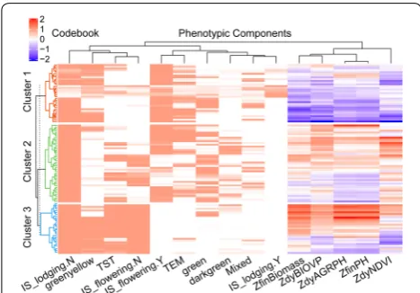
Finally, we ran SOM with the following parameters according to the guidelines for building a SOM reported by Das [51] and Wendel [52] : SOM size: 15 × 7; 5000 iterations; learning rate: 0.05, hexagonal topology and Gaussian neighborhood function. We resolved the clus-ters derived from the SOM map into a set of clustering rules by using the rpart [53] (version 4.1-15) and rpart. plot [54] (version 3.0.7) R package and evaluated tering quality. To facilitate interpretation of the clus-ters, we used the ComplexHeatmap R package (version 1.99.5) [55] to enhance the visualization of the cluster-ing results by makcluster-ing a heat map with a dendrogram. The UpSetR R package (version 1.3.3) [56] used to visu-alize the set intersections was also used to identify clus-ters with typical phenotypic-component patterns.
Wilcoxon rank-sum test was used to compare each cluster mean with the total population (without clus-tering) mean, and observe whether a phenotypic com-ponent was overexpressed (above the total population mean) or underexpressed (below the total popula-tion mean) in different clusters.
Analysis of principle components analysis bioplot
Two-step clustering was followed by biplot analysis associated with principle components analysis (PCA). By using the FactoMineR [57] and factoextra [58] R packages, the biplot was analyzed with a new dataset based on two-step clustering to characterize the rela-tionship between phenotypic components and to iden-tify the leading components. Biplots based on simple bivariate scatter plots can show inter-unit distances and indicate clustering of units in addition to display-ing variances in and correlations between the variables [59]. The new dataset was projected onto two dimen-sions to approximately preserve the distances between the samples. The points in the biplot approximate the row (sample) information and the vector approximates the column (i.e., phenotypic component) information. The distance between points reflects the difference between the corresponding samples. A greater dis-tance between two points reflects a greater difference between the corresponding samples, and vice versa. The length of the arrows represents how well the phe-notypic component explains the distribution of the data, whereas the angles between the arrows approxi-mate their correlations. Therefore, when two vec-tors are approximately perpendicular, the correlation between the two variables is very weak, and they are essentially independent of each other. But if they are nearly parallel (antiparallel), the variables have a high positive (negative) correlation.
Results
Phenotypic components from high‑throughput phenotyping images
The phenotypic components evaluated in this study included plant height, fresh biomass, flowering, lodg-ing, leaf color, genetic background, NDVI, AGRPH and BIOVP. Except for genetic background, these phe-notypic components were acquired by processing and analyzing digital or multispectral images from HTP. Manual grading based on field investigations led to extreme imbalance of the lodging samples, i.e., more than 80% was root lodging [29]. Therefore, we simply divided the population into two categories (i.e., lodg-ing and non-lodglodg-ing). Note that NDVI, BIOVP, and AGRPH were all time series data. For convenience, we converted the time series data into a numerical value by calculating the area under the polyline (Fig. 4). Phe-notypic components were classified into three catego-ries based on data types: numerical, dichotomous, and polytomous. Table 3 summarizes the phenotypic data evaluated in this study.
Clustering genotypes based on phenotypic components
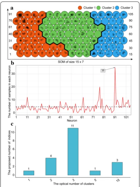
There were five input data layers. The numerics layer consisted of five continuous numerical variables (i.e., dyAGRPH, dyNDVI, dyBIOVP, finBiomass and finPH, see Table 3). Figure 5 shows that the relative dis-tance to the closest unit approximately stabilizes after 5000 iterations, which means that the algorithm has converged. A total of 105 neurons in the SOM were arranged in a grid of 15 rows by 7 columns, and 482 samples were unevenly distributed among these neu-rons (Fig. 6a). Samples with similar phenotypic-com-ponent patterns tended to be at nearby grid locations. The 91st neuron contained 35 samples, which was the largest number of samples for a single neuron. Seven neurons, called “dead” neurons, never won the com-petition for samples; these accounted for less than 7% (Fig. 6b). Figure 6c shows that, based on the majority rule, 11 of the 20 indices propose three as the optimal number of clusters. In other words, these phenotypic components contributed strongly to discrimination of genotypes into three clusters. Therefore, hierarchical
agglomerative clustering of 105 codebooks resulted in the identification of three major clusters, with differ-ent genotype samples assigned to these clusters (Fig. 7). After clustering, genotypes with similar phenotypic-component characteristics were grouped in the same cluster. The next section discussed co-expressed geno-types and how to identify plant phenotypic similarity.
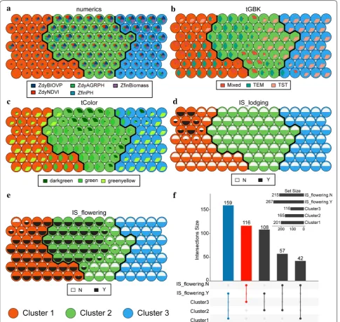
Phenotypic map and similarity
A phenotypic map was constructed by using SOM clus-tering visualization technology and dendrograms. This map provides important information regarding plant phenotypic similarity or dissimilarity and supports fur-ther evaluation of the phenotypic components [28]. By visualizing the weight vector on the map, we explored the patterns in which the samples and phenotypic com-ponents distributed across the three clusters. The weight vector was visualized as a “fan diagram” to indicate the weight of each phenotypic component in a neuron (see Figs. 8a–e). Closer inspection of these diagrams shows that (i) the weights of the numerical phenotypic compo-nents are relatively small in cluster 1 (Fig. 8a); (ii) the TST subpopulation dominates cluster 3, accounting for more than 85% (Fig. 8b); (iii) cluster 2 has almost no green-yellow samples (less than 5% of the samples), although Fig. 4 Converting time series data (BIOVP) into a numerical value
by calculating the area under the polyline. The first five plots were selected as examples. The number in the right column indicated the corresponding area after conversion
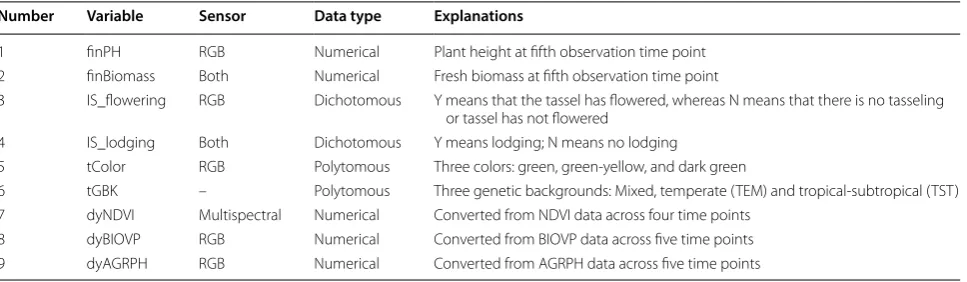
Table 3 Phenotypic components evaluated in this study
Number Variable Sensor Data type Explanations
1 finPH RGB Numerical Plant height at fifth observation time point
2 finBiomass Both Numerical Fresh biomass at fifth observation time point
3 IS_flowering RGB Dichotomous Y means that the tassel has flowered, whereas N means that there is no tasseling or tassel has not flowered
4 IS_lodging Both Dichotomous Y means lodging; N means no lodging
5 tColor RGB Polytomous Three colors: green, green-yellow, and dark green
6 tGBK – Polytomous Three genetic backgrounds: Mixed, temperate (TEM) and tropical-subtropical (TST) 7 dyNDVI Multispectral Numerical Converted from NDVI data across four time points
8 dyBIOVP RGB Numerical Converted from BIOVP data across five time points
9 dyAGRPH RGB Numerical Converted from AGRPH data across five time points
they accounted for over 75% of the samples in cluster 3 (Fig. 8c); (iv) all samples containing lodging phenotypic components are in cluster 1 (Fig. 8d); and (v) none of the samples in cluster 3 are tasseling and flowering (Fig. 8e).
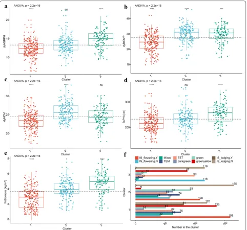
As shown in Fig. 9, the overall analysis of variance (ANOVA) gives a p value less than 0.05, so we further compared the differences in the mean phenotypic com-ponents between each cluster and that of all genotypes without clustering. When the Wilcoxon rank-sum test was significant, the numerical phenotypic components in cluster 1 were significantly low compared with all components (i.e., without clustering), and other numeri-cal phenotypic components except dyNDVI in Cluster 3 were significantly higher compared to all components. However, no significant difference appeared in the parameters finPH and dyNDVI between cluster 2 and all components. Phenotypic components with similar char-acteristics were considered to be co-expressed by differ-ent genotypes. Together, the visualization of the results of the analysis provided important insights into the clusters
and their co-expressed patterns based on two-step clus-tering (Table 4).
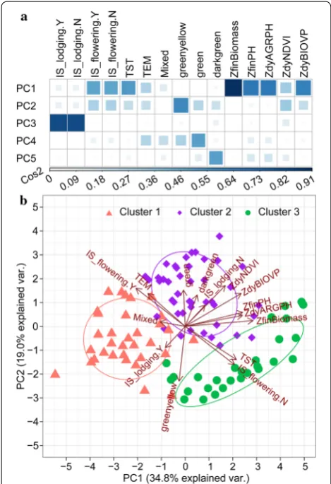
Turning now to phenotypic similarity, Fig. 7 provides an overview, via a dendrogram, of the measurement of the similarity between phenotypic components by using HAC with the spearman correlation distance. The top five principal components (PCs) explained 86.2% of the variation. A high Cos2 (square cosine, squared coordi-nates) indicates that the phenotypic component is well represented in the principal component [58]. Therefore, ZfinBiomass (i.e., standardized fresh biomass) was more important to interpret PC 1, and IS_lodging was more important to interpret PC 3 (Fig. 10a). Figure 10b pre-sents a biplot that simultaneously plots information on genotype samples and phenotypic components, further revealing the phenotypic similarity and the relationship between genotypes and phenotypic components. PC 1 explained 34.8% of the variation and PC 2 explained 19.0% of the variation. A high positive correlation existed between the numerical phenotypic components, which were negatively correlated with IS_lodging.Y. Lodging had a negative impact on crop biomass, plant height, NDVI, and so on. A significant positive correlation occurred between TST and IS_flowering.N and between TEM and IS_flowering.N, which we attributed to the fact that the experimental site was located in a temperate zone, so the TEM subpopulation was tasseling and flowering in the V1 stage, whereas the TST subpopulation required more accumulated temperature from vegetative overgrowth to reproductive growth. The correlation between greenyel-low and IS_lodging.Y was interesting because it seemed to indicate that the green-yellow leaf samples were more prone to lodging. Similarly, a significant positive cor-relation occurred between darkgreen and ZdyNDVI. Interestingly, this correlation was related to the canopy pigment content, which was remotely estimated based on the NDVI.
Discussion
Phenotypic temporal profile
Prior studies noted the importance of phenotypic tem-poral profiles, providing fresh insights into the dynamic changes in phenotypic traits [15, 60] and genetic differ-ences at various stages of plant development [27, 61]. Although UAV-HTP allows researchers to efficiently and conveniently acquire multi-temporal phenotypic data by remote sensing, integrating time-series data with other types of phenotypic data, such as leaf color, to facili-tate subsequent quantitative genetic analysis remains a difficult problem. In this study, the area under the polyline is highly correlated with other phenotypic com-ponents after conversion to a single value (Figs. 3 and 10). Although this conversion preserves the multi-temporal Fig. 6 Frequency distribution of samples in SOM grid and optical
information of phenotypic components to some extent, obvious deficiencies remain because, given equal areas, the shape of the polylines may differ. This leaves the way open for further improvements: one option would be to add some descriptive parameters such as inflection points and trends. The challenges of collecting pheno-typic temporal profiles are further compounded by their observed values, which partially depend on environ-mental conditions and may change dramatically within a given day or between days of a given year [36].
Phenotypic preselection
The results of this study show that two-step clustering allows genotypes to be segregated according to different phenotypic component patterns. For example, cluster 3 exhibits a pattern that is a higher numerical phenotypic components, so when we preliminarily screen genotypes for higher biomass or higher plant height, which are both key breeding targets for crop improvement, we can nar-row the range of candidate populations and select geno-types only in this cluster. Grain yield is also one of the most important breeding targets for breeders. Unfortu-nately, the grain-yield data for this trial were largely miss-ing and unreliable due to waterloggmiss-ing caused by heavy rainfall during the harvest period. These data were there-fore replaced by the historical grain-yield data. In this way, we try to further explain the rationality of clustering results produced by our pre-selection framework.
in cluster 3 are TST subpopulations planted in the tem-perate zone, where the grain yield of such TST popula-tions was low due to the lack of sufficient accumulated temperature during the reproductive-growth stage. Grain yield is a polygenic trait controlled by several genes [62]; phenotypic components do not directly affect the yield but assist in the identification of the genotypes.
Phenotypes of a plant are the expression in observable traits of potential genes comprising the genotype and are determined by its genetic composition, the environment in which it grows, and the interactions between genotype and environment [63, 64]. It is thus possible to measure phenotypic relationships between different genotypes based on available traits [28]. Some phenotypic data extracted from remote sensing images, such as BIOVP and NDVI, clearly differ from the agronomic definition, or “trait.” To distinguish between them, we refer herein to these phenotypic data as phenotypic components. The analysis of phenotypic similarity provides a new inspira-tion that removes some highly relevant phenotypic com-ponents and thereby reduces data redundancy. In other words, the workload can be reduced by making a prelimi-narily selection of representative phenotypic components as the research objects in the trial design.
Limitations and Implications of Study
According to the literature, SOM does not really clus-ter but instead produces a reduced representation of the original data set [46]. Because SOM lacks hierarchical structure, it is impossible to detect higher-order relation-ships between clusters. In this study, we demonstrate a two-step clustering method that combines hierarchical clustering and self-organizing maps to cluster, analyze, and visualize the mixed continuous and categorical data, providing a very efficient tool for exploratory analysis of genotype co-expression and phenotypic similarity. One problem with self-organizing maps is the occurrence of dead neurons, whose randomly initialized weight vec-tors farther from any data point prevent them from ever being chosen as BMU, which degrades the learning effi-ciency. Therefore, if the percentage of dead neurons is large, caution must be applied and the grid size of SOM should be readjusted. After resolving the clusters derived from the SOM map reasonably to a set of clustering rules, Fig. 7 Hierarchical agglomerative clustering for codebook. Clustering
approximately 95.2% of the samples can be accurately predicted by using a decision tree. However, the cluster-ing boundaries are not 100% sharp, and some ambiguity remains regarding where on the map a specific neuron (sample) migrates (Fig. 12).
The challenge for plant breeders is to identify and select the plants with the target phenotype controlled
conditions were attained by doing single-factor experi-ments and using uniform field-management practices. Even so, the explanation for these results may be the lack of adequate verification, because these phenotypic components were acquired and analyzed only across a single growing season. Further research should be undertaken to investigate the population and provide new multi-year insights into identifying genotypes and
their co-expressed patterns and selecting phenotypic similarity.
at the late ripening stage prevented the formation of a phenotypic data chain throughout growing season. A hyperspectral sensor is a powerful tool for detecting biological and abiotic stresses, and more crop resist-ance information can be obtained when it is loaded on the UAV platform. The platform will also be improved to increase payload capacity so that it may be equipped with UAV laser scanning for easy access to plant type and ear-high traits. The phenotypic map and simi-larity will also more comprehensive when more data from UAV laser scanning and hyperspectral sensor are available. Rich phenotypic data definitely assist breed-ers with identifying and selecting the best candidate genotypes.
Table 4 Summary of clusters and their co-expressed patterns based on two-step clustering
Cluster Neuron size Sample size Description
1 33 201 Lower numerical phenotypic components, e.g., less fresh biomass and lower average
growth rate of plant height
2 44 165 Green or dark green leaves, almost no green-yellow leaves
Larger NDVI
3 28 116 Higher numerical phenotypic components, e.g., more fresh biomass and plant height
Longer vegetative growth stage
Fig. 10 PCA biplot showing phenotypic similarity and relationship between genotypes and phenotypic components. a Visualization of quality of representation of variables in top five dimensions.
Cos2 is the quality of representation of the variables in the principal component maps. b Biplot analysis for phenotypic similarity. Correlated phenotypic components and genotype samples were located in the same quadrant. The cosine of the angle between vectors indicated correlation between phenotypic components. Highly correlated phenotypic components pointed in roughly the same direction. Nearby points in the biplot represented samples with similar patterns; these were colored according to clustering. The initial letter “Z” indicated that this variable is standardized
Conclusions
In this study, we collected for a maize breeding program a short time series of remote-sensing images, including digital and multispectral images, by using an UAV-based HTP platform. The images were used to acquire nine phenotypic components. Here, we propose a framework for pre-screening genotypes and phenotypes based on HTP phenotypic components. The core procedure of this framework can be summarized as follows: we use two-step clustering to identify co-expressed patterns, and then pre-select genotypes. We then use correlation analysis to analyze phenotypic similarity, and then pre-select phenotypic components. This framework gives breeders additional information to quickly identify and select plants that have genotypes that confer desirable phenotypic components from thousands of field plots. The present study also demonstrates that remote sensing is a powerful tool that provides an opportunity to acquire abundant phenotypic components. By using these rich phenotypic components, breeders should be able to more effectively identify and select superior genotypes.
Additional file
Additional file 1. Twenty indices for determining the best number of clusters.
Abbreviations
AGRPH: average growth rate of plant height; AHC: agglomerative hierarchical clustering; ANOVA: analysis of variance; AOI: area of interest; BIOVP: a volume metric used to estimate crop biomass within a plot; Cos2: square cosine and squared coordinates; CSM: crop surface model; DAS: days after sowing; DSM: digital surface model; DEM: digital elevation model; DSMs: digital surface models; HTP: high-throughput phenotyping; NGRDI: normalized green–red difference index; NDVI: normalized difference vegetation index; PCA: principle components analysis; SOM: self-organizing map; UAV: unmanned aerial vehi-cle; VIs: vegetation indices.
Acknowledgements
We thank the Maize Research Center department of the Beijing Academy of Agriculture and Forestry Sciences for preparing the seed and planting for the trial, and Dr. Yanxin Zhao, Dr. Xiaqing Wang, and Mr. Ruyang Zhang for designing the experiments and helping to collect the field data. We are also grateful to the anonymous reviewers for their valuable comments and recommendations.
Authors’ contributions
LH drafted and revised the manuscript. GY and CZ proposed the conceptual-ization of this study and reviewed the manuscript. HD edited the manuscript. HY and LH performed field experiments. BX collected image data. LH, ZL and XY analyzed and interpreted the results. HL and HL assisted in develop-ing analysis methods and in revisdevelop-ing the manuscript. All authors read and approved the final manuscript.
Funding
This study was supported by the National Key Research and Development Program of China (2017YFE0122500), the Natural Science Foundation of China (41771469), the Beijing Natural Science Foundation (6182011), and the Special Funds for Technology innovation capacity building sponsored by the Beijing Academy of Agriculture and Forestry Sciences (KJCX20170423).
Availability of data and materials
The datasets analysed during the current study are available from the cor-responding author on reasonable request.
Ethics approval and consent to participate Not applicable.
Consent for publication Not applicable.
Competing interests
The authors declare that they have no competing interests.
Author details
1 Key Laboratory of Quantitative Remote Sensing in Agriculture of Ministry of Agriculture, Beijing Research Center for Information Technology in Agricul-ture, Beijing 100097, China. 2 College of Architecture and Geomatics Engineer-ing, Shanxi Datong University, Datong 037003, China. 3 National Engineering Research Center for Information Technology in Agriculture, Beijing 100097, China. 4 College of Geoscience and Surveying Engineering, China University of Mining and Technology (Beijing), Beijing 100083, China.
Received: 29 March 2019 Accepted: 22 May 2019
References
1. Furbank RT, Tester M. Phenomics—technologies to relieve the phenotyp-ing bottleneck. Trends Plant Sci. 2011;16(12):635–44.
2. Ninomiya S, Baret F, Cheng Z-MM. Plant phenomics: emerging transdis-ciplinary science. Plant Phenom. 2019;2019:1–3. https ://doi.org/10.34133 /2019/27651 20.
3. The UN Food and Agriculture Organisation (FAO). How to Feed the World in 2050. 2009: Rome. p. 35.
4. Yang G, Liu J, Zhao C, Li Z, Huang Y, Yu H, Xu B, Yang X, Zhu D, Zhang X, Zhang R, Feng H, Zhao X, Li Z, Li H, Yang H. Unmanned aerial vehicle remote sensing for field-based crop phenotyping: current status and perspectives. Front Plant Sci. 2017;8:1111.
5. Cobb JN, DeClerck G, Greenberg A, Clark R, McCouch S. Next-generation phenotyping: requirements and strategies for enhancing our under-standing of genotype-phenotype relationships and its relevance to crop improvement. Theor Appl Genet. 2013;126(4):867–87.
6. Araus JL, Cairns JE. Field high-throughput phenotyping: the new crop breeding frontier. Trends Plant Sci. 2014;19:52–61.
7. Campbell ZC, Acosta-Gamboa LM, Nepal N, Lorence A. Engineering plants for tomorrow: how high-throughput phenotyping is contributing to the development of better crops. Phytochem Rev. 2018;17:1329–43. 8. Fernandez MGS, Bao Y, Tang L, Schnable PS. A high-throughput,
field-based phenotyping technology for tall biomass crops. Plant Physiol. 2017;174(4):2008–22.
9. Araus JL, Kefauver SC, Zaman-Allah M, Olsen MS, Cairns JE. Translat-ing high-throughput phenotypTranslat-ing into genetic gain. Trends Plant Sci. 2018;23(5):451–66.
10. Crain JL, Wei Y, Barker J, Thompson SM, Alderman PD, Reynolds M, Zhang NQ, Poland J. Development and deployment of a portable field pheno-typing platform. Crop Sci. 2016;56(3):965–75.
11. Bai G, Ge YF, Hussain W, Baenziger PS, Graef G. A multi-sensor system for high throughput field phenotyping in soybean and wheat breeding. Comput Electron Agric. 2016;128:181–92.
12. White JW, Andrade-Sanchez P, Gore MA, Bronson KF, Coffelt TA, Conley MM, Feldmann KA, French AN, Heun JT, Hunsaker DJ, Jenks MA, Kimball BA, Roth RL, Strand RJ, Thorp KR, Wall GW, Wang G. Field-based phenom-ics for plant genetphenom-ics research. Field Crops Res. 2012;133:101–12. 13. Ludovisi R, Tauro F, Salvati R, Khoury S, Mugnozza Scarascia G, Harfouche
A. UAV-based thermal imaging for high-throughput field phenotyping of black poplar response to drought. Front Plant Sci. 2017;8:1681-81. 14. Maimaitijiang M, Ghulam A, Sidike P, Hartling S, Maimaitiyiming M,
Peterson K, Shavers E, Fishman J, Peterson J, Kadam S, Burken J, Fritschi F. Unmanned Aerial System (UAS)-based phenotyping of soybean using multi-sensor data fusion and extreme learning machine. ISPRS J Photo-gramm Remote Sens. 2017;134:43–58.
15. Han L, Yang G, Yang H, Xu B, Li Z, Yang X. Clustering field-based maize phenotyping of plant-height growth and canopy spectral dynamics using a UAV remote-sensing approach. Front Plant Sci. 2018;9:1638.
16. Haghighattalab A, Perez LG, Mondal S, Singh D, Schinstock D, Rutko-ski J, Ortiz-Monasterio I, Singh RP, Goodin D, Poland J. Application of unmanned aerial systems for high throughput phenotyping of large wheat breeding nurseries. Plant Methods. 2016;12:15.
17. Deng L, Mao Z, Li X, Hu Z, Duan F, Yan Y. UAV-based multispectral remote sensing for precision agriculture: a comparison between different cam-eras. ISPRS J Photogramm Remote Sens. 2018;146:124–36.
18. Khan Z, Rahimi-Eichi V, Haefele S, Garnett T, Miklavcic SJ. Estimation of vegetation indices for high-throughput phenotyping of wheat using aerial imaging. Plant Methods. 2018;14(1):20.
19. Aasen H, Honkavaara E, Lucieer A, Zarco-Tejada PJ. Quantitative remote sensing at ultra-high resolution with UAV spectroscopy: a review of sensor technology, measurement procedures, and data correction work-flows. Remote Sens. 2018;10(7):1091.
20. Ampatzidis Y, Partel V. UAV-based high throughput phenotyping in citrus utilizing multispectral imaging and artificial intelligence. Remote Sens. 2019;11(4):410.
21. Han L, Yang G, Dai H, Xu B, Yang H, Feng H, Li Z, Yang X. Modeling maize above-ground biomass based on machine learning approaches using UAV remote-sensing data. Plant Methods. 2019;15(1):10.
22. Crain J, Reynolds M, Poland J. Utilizing high-throughput phenotypic data for improved phenotypic selection of stress-adaptive traits in wheat. Crop Sci. 2017;57(2):648–59.
23. Duan T, Chapman SC, Guo Y, Zheng B. Dynamic monitoring of NDVI in wheat agronomy and breeding trials using an unmanned aerial vehicle. Field Crops Res. 2017;210:71–80.
24. Zhang XH, Huang CL, Wu D, Qiao F, Li WQ, Duan LF, Wang K, Xiao YJ, Chen GX, Liu Q, Xiong LZ, Yang WN, Yan JB. High-throughput phenotyping and QTL mapping reveals the genetic architecture of maize plant growth. Plant Physiol. 2017;173(3):1554–64.
25. Watanabe K, Guo W, Arai K, Takanashi H, Kajiya-Kanegae H, Kobayashi M, Yano K, Tokunaga T, Fujiwara T, Tsutsumi N, Iwata H. High-throughput phenotyping of sorghum plant height using an unmanned aerial vehicle and its application to genomic prediction modeling. Front Plant Sci. 2017;8:11.
26. Hu P, Chapman SC, Wang X, Potgieter A, Duan T, Jordan D, Guo Y, Zheng B. Estimation of plant height using a high throughput phenotyping platform based on unmanned aerial vehicle and self-calibration: example for sorghum breeding. Eur J Agron. 2018;95:24–32.
27. Pugh NA, Horne DW, Murray SC, Carvalho G, Malambo L, Jung J, Chang A, Maeda M, Popescu S, Chu T, Starek MJ, Brewer MJ, Richardson G, Rooney WL. Temporal estimates of crop growth in sorghum and maize breeding enabled by unmanned aerial systems. Plant Phenome J. 2018;1(1):170006. 28. Chen D, Neumann K, Friedel S, Kilian B, Chen M, Altmann T, Klukas C.
Dissecting the phenotypic components of crop plant growth and drought responses based on high-throughput image analysis. Plant Cell. 2014;26(12):4636–55.
29. Han L, Yang G, Feng H, Zhou C, Yang H, Xu B, Li Z, Yang X. Quantitative identification of maize lodging-causing feature factors using unmanned aerial vehicle images and a nomogram computation. Remote Sens. 2018;10(10):1528.
30. Liu T, Li R, Zhong X, Jiang M, Jin X, Zhou P, Liu S, Sun C, Guo W. Estimates of rice lodging using indices derived from UAV visible and thermal infra-red images. Agric For Meteorol. 2018;252:144–54.
31. Friedman JM, Hunt ER, Mutters RG. Assessment of leaf color chart obser-vations for estimating maize chlorophyll content by analysis of digital photographs. Agron J. 2016;108(2):822–9.
32. Vergara-Diaz O, Zaman-Allah MA, Masuka B, Hornero A, Zarco-Tejada P, Prasanna BM, Cairns JE, Araus JL. A novel remote sensing approach for prediction of maize yield under different conditions of nitrogen fertiliza-tion. Front Plant Sci. 2016;7:666.
33. Naito H, Ogawa S, Valencia MO, Mohri H, Urano Y, Hosoi F, Shimizu Y, Chavez AL, Ishitani M, Selvaraj MG, Omasa K. Estimating rice yield related traits and quantitative trait loci analysis under different nitrogen treatments using a simple tower-based field phenotyping system with modified single-lens reflex cameras. ISPRS J Photogramm Remote Sens. 2017;125:50–62.
•fast, convenient online submission •
thorough peer review by experienced researchers in your field
• rapid publication on acceptance
• support for research data, including large and complex data types
•
gold Open Access which fosters wider collaboration and increased citations maximum visibility for your research: over 100M website views per year •
At BMC, research is always in progress.
Learn more biomedcentral.com/submissions
Ready to submit your research? Choose BMC and benefit from: cultivars. BMC Genet. 2018;19(1):8.
38. Oyelade J, Isewon I, Oladipupo F, Aromolaran O, Uwoghiren E, Ameh F, Achas M, Adebiyi E, Clustering algorithms: their application to gene expression data. Bioinform Biol Insights 2016. 10: p. BBI.S38316. 39. Higuera C, Gardiner KJ, Cios KJ. Self-organizing feature maps identify
proteins critical to learning in a mouse model of down syndrome. PLoS ONE. 2015;10(6):e0129126.
40. Kohonen T. Automatic formation of topological maps in a self-organizing system. In Proceedings of the Scandinavian Conference on Image Analy-sis. 1981.
41. Kohonen T. Exploration of very large databases by self-organizing maps. In Proceedings of International Conference on Neural Networks (ICNN’97). 1997.
42. Augustijn E-W, Zurita-Milla R. Self-organizing maps as an approach to exploring spatiotemporal diffusion patterns. Int J Health Geogr. 2013;12:60–61.
43. Bro R, Smilde AK. Principal component analysis. Anal Methods. 2014;6(9):2812–31.
44. Ritchie S W, Hanway J J, and Benson G O, How a corn plant develops, in Special Report #48. 1993, Iowa State University of Science and Technol-ogy Cooperative Extension Service: Ames, IA, USA.
45. Agisoft. Orthophoto & DEM Generation (with GCPs). 2018 [cited 2018 19 October,2018]. http://www.agiso ft.com/suppo rt/tutor ials/begin ner-level /.
46. Herrero J, Dopazo J. Combining hierarchical clustering and self-organiz-ing maps for exploratory analysis of gene expression patterns. J Proteome Res. 2002;1(5):467–70.
47. Wehrens R, Buydens LMC. Self- and super-organizing maps in R: The kohonen Package. J Stat Softw. 2007;21(5):19.
48. Algobeans. Self-organizing maps tutorial. n.d. [cited 2019 January, 12].
https ://algob eans.com/2017/11/02/self-organ izing -map/.
49. Charrad M, Ghazzali N, Boiteau V, Niknafs A. NbClust: an R package for determining the relevant number of clusters in a data set. J Stat Softw. 2014;61(6):36.
50. Yang Y. Ensemble learning. In: Yang Y, editor. temporal data mining via unsupervised ensemble learning. Amsterdam: Elsevier; 2017. p. 35–56. 51. Das G, Chattopadhyay M, Gupta S. A comparison of self-organising maps
and principal components analysis. Int J Market Res. 2016;58(6):815–34.
56. Lex A, Gehlenborg N, Strobelt H, Vuillemot R, Pfister H. UpSet: visualization of Intersecting Sets. IEEE Trans Visual Comput Graphics. 2014;20(12):1983–92.
57. Sebastien L, Julie J, Francois H. FactoMineR: an R package for multivariate analysis. J Stat Softw. 2008;25:1–8.
58. Alboukadel K, Practical Guide to Principal Component Methods in R. 2018. 59. Gabriel KR. The biplot graphic display of matrices with application to
principal component analysis. Biometrika. 1971;58(3):453–67. 60. Potgieter A B, George-Jaeggli B, Chapman S C, Laws K, Suárez Cadavid
L A, Wixted J, Watson J, Eldridge M, Jordan D R, and Hammer G L, Multi-spectral imaging from an unmanned aerial vehicle enables the assess-ment of seasonal leaf area dynamics of sorghum breeding lines. Front Plant Sci. 2017;8(1532).
61. Cooper M, Messina CD, Podlich D, Totir LR, Baumgarten A, Hausmann NJ, Wright D, Graham G. Predicting the future of plant breeding: comple-menting empirical evaluation with genetic prediction. Crop Pasture Sci. 2014;65(4):311–36.
62. Mendes-Moreira P, Alves ML, Satovic Z, Dos Santos JP, Santos JN, Souza JC, Pêgo SE, Hallauer AR, Vaz Patto MC. Genetic architecture of ear fasciation in maize (Zea mays) under QTL scrutiny. PLoS ONE. 2015;10(4):e0124543-e43.
63. Walter A, Liebisch F, Hund A. Plant phenotyping: from bean weighing to image analysis. Plant Methods. 2015;11:14.
64. Dhondt S, Wuyts N, Inze D. Cell to whole-plant phenotyping: the best is yet to come. Trends Plant Sci. 2013;18(8):433–44.
65. Hopkins AA, Saha MC, Wang ZY. Breeding, genetics, and cultivars, in tall fescue for the twenty-first century. Fribourg HA, Hannaway DB, West CP, Editors. 2009, American Society of Agronomy.
66. Crain J, Mondal S, Rutkoski J, Singh RP, Poland J. Combining high-throughput phenotyping and genomic information to increase prediction and selection accuracy in wheat breeding. Plant Genome 2018;11(1):1–14.
Publisher’s Note