551 Information Technology and Control 2018/3/47
Self-Tuning Method of PID
Parameters Based on Belief Rule
Base Inference
ITC 3/47
Journal of Information Technology and Control
Vol. 47 / No. 3 / 2018 pp. 551-563
DOI 10.5755/j01.itc.47.3.19045 © Kaunas University of Technology
Self-Tuning Method of PID Parameters Based on
Belief Rule Base Inference
Received 2017/09/14 Accepted after revision 2018/07/26
http://dx.doi.org/10.5755/j01.itc.47.3.19045
Corresponding author: [email protected]; tel.: +86-150-8878-3292
Xiao-Bin Xu, Xue Ma, Cheng-Lin Wen
School of Automation, Hangzhou Dianzi University, Hangzhou, China
Da-Rong Huang
School of Information Science and Engineering, Chongqing Jiaotong University, Chongqing, 40074, China
Jian-Ning Li
School of Automation, Hangzhou Dianzi University, Hangzhou, China
As a generic inference mechanism, the belief rule-based (BRB) system can effectively integrate quantitative in-formation with qualitative knowledge to model causal relationships of complex application systems. Based on the BRB, this paper develops a novel self-tuning strategy of PID parameters such that the output of closed-loop control system generated by PID controller can accurately follow control input. Firstly, the initial belief rule base is abstracted from expert’s control experiences to depict the highly nonlinear relationship between the variables of control system and each PID parameter. Secondly, the objective function is established to minimize the error between the given control input and the closed loop output, and then the online optimization method via sequen-tial linear programming is presented to optimize the parameters of BRB system so as to adaptively adjust PID parameters by the optimized BRB system in real time. Typical control simulation experiments of DC motor are implemented to illustrate the advantages of the proposed BRB-PID over widely used neural network-based PID.
KEYWORDS: Belief Rule Base (BRB), PID controller, Sequential linear programming (SLP) algorithm, Evi-dence Reasoning(ER).
1. Introduction
PID is one of the earliest control strategies proposed in classical control theory, which has been widely used in industrial control systems and achieved good
appro-Information Technology and Control 2018/3/47 552
priate selection of PID parameters. Hence, in order to obtain the satisfactory control effect, one has to study on available methods for determining the val-ue of PID parameters, which are the key link in the design of PID controller, and what’s more, with the increasing complexities of the structures, functions and operating conditions of controlled objects, this issue becomes more and more important for appli-cations of PID strategy [17]. So experts and scholars have been concentrating on the self-tuning methods for PID parameters, so that the adaptive PID control could be chosen to adapt to the complex and change-able controlled objects, and meet the control require-ments with high performance and high precision [16]. In essence, these methods all attempt to explore ap-propriate models to establish a nonlinear mapping re-lationship between the variables of a control system (including the given input, actual output, deviation and the deviation change rate, etc) and PID param-eters (the proportional, integral, differential coeffi-cients KP, KI, KD, respectively), also there exists
var-ious uncertainties in this mapping relationship due to the complexity of controlled objects and various disturbances [8].
Nowadays, artificial intelligence methods have been widely used to turn or set PID parameters adaptive-ly, which greatly enhance tuning effect and efficiency [2], mainly including Expert system-based PID (ES-PID), Fuzzy inference-based PID (FI-PID) and Arti-ficial neural network-based PID (ANN-PID) etc. ES-PID abstracts heuristic rules from expert’s knowledge about controlled object and control experience to de-pict the nonlinear relationship between the control variables and PID parameters, and then, the designed inference engine can infer the corresponding values of PID parameters from the rules activated by the on-line values of control variables[9]. However, there are some difficult issues one has to face, such as, how to distinguish good knowledge from bad knowledge be-cause the latter will lead to useless, conflicting, even counter-intuitive rules; how to enhance the online learning and updating abilities of expert system and improve completeness and adaptability of the con-structed rule base [13]. In order to deal with fuzzy uncertainty of human knowledge, FI-PID introduces the fuzzy rules to model the imprecise relationship between the control variables and PID parameters, and then uses the fuzzy inference engine to adjust the
values of PID parameters [7]. Comparing with tradi-tional ES-PID, FI-PID can capture more useful infor-mation with uncertainty in expert’s knowledge and has better generalization capability. However, simi-lar with ES-PID, it also suffers from some difficulties including poor online learning and updating abilities and incompleteness of fuzzy rule base and so on [10]. ANN-PID uses the hidden layer network structure to construct the connection between the input layer (control variables) and the output layer (PID parame-ters), and online optimizes network weights to obtain desired values of PID parameters which is a kind of typical adaptive PID control [20]. However, the neural network is a black box system, in which, the physical meanings of network nodes are obscure and even hard to understand for control engineers. Although, when objective functions are given, so many optimization strategies can be used to online adjust the networks weights, the optimized results are easy to fall into local minimum in training process because of the improper initial values of weights or other reasons [15].
553 Information Technology and Control 2018/3/47
so on) are considered in ER fusion process [3]; (3) compared with neural network, the physical mean-ings of the parameters in BRB (value and weight of attribute, belief distribution, rule weight, etc.) are not obscure, but very clear and easy to be understood by control engineers. Therefore, they can adjust BRB system according to themselves intentions. These parameters can also be trained and optimized using available methods. Therefore, the BRB methodology has attracted wide attentions in various industrial applications including alarm monitoring, fault diag-nosis, risk and decision analysis and so on [21, 24]. This paper aims to design a novel adaptive BRB-PID controller to deal with self-tuning of PID parameters. Firstly, the initial belief rule base is abstracted from expert’s control experiences to describe the high-ly nonlinear relationships between the variables of control system and PID parameters. Secondly, in or-der to reflect the real-time changes of this nonlinear relationship with sampling time, the online optimi-zation method via sequential linear programming is presented to optimize the parameters of BRB system, and then the optimized BRB can adaptively reason out the values of PID parameters such that the output of closed-loop control system generated by the proposed adaptive BRB-PID controller can accurately follow the given input. The typical control experiments of DC mo-tor are implemented to illustrate the advantages of the proposed adaptive BRB-PID control over the widely used adaptive neural network-based PID control.
2. Self-Tuning of PID Parameters via
BRB Inference
2.1. Incremental PID Control
The well-known discrete-time incremental PID con-troller can be expressed as [18]:
( ) ( 1) ( ( ) ( 1)) ( ( ) ( 1)) 2
+ ( ( ) 2 ( 1) ( 2)), 2
I P
D
K T
u k u k K e k e k e k e k
K T e k e k e k
= - + - - + +
-- - +
-(1)
where e(k)= r(k)-y(k) is the deviation that the closed-loop output y(k) tracks the given input (the desired
closed-loop output) r(k). u(k) is the control effort at time step k. KP, KIand KD are proportional, integral
and derivative gains, respectively. T is the sampling period. From (1), the increment can be given as
( ) ( ) ( 1) P P( ) I I( ) D D( ),
u k u k u k K e k K e k K e k
Δ = - - = + + (2)
where eP =e k e k( ) ( 1),- - eI =T e k e k( ( ) ( 1)) / 2,+
-( -( ) 2 -( 1) -( 2)) /
D
e = e k - e k- +e k- T .
2.2. The Design of BRB-PID Controller
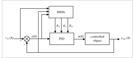
Fig. 1 shows the structure of BRB-PID controller, in which, PID has the incremental form as given in (1). The values of the parameters KP, KI and KD can be
online estimated by, respectively, constructed three BRBs with the same inputs (rin, e, yout) and the
differ-ent outputs (KP,KI, KD). The whole modeling and
in-ference procedure can be described as follows. First-ly, based on the expert’s control experiences, we can construct BRB models which consist of rules and their parameters including the reference valued of the input variables rin, e, yout (antecedent attributes),
the output variables KP, KI and KD (consequent
hy-pothesis) and the values of rule weights and attribute weights; secondly, when the input data are online ob-tained, they are inputted into the BRB models, and then the activated rules and the corresponding acti-vation weights can be acquired. The ER algorithm is used to fuse the consequent belief distributions of the activated rules. The values of PID parameters can be estimated from the fused belief distribution via utili-ty principle [1]. In this inference process, it should be noted that we must online optimize the parameters of BRB such that the error between the closed loop output deduced from BRB-PID and the control input is minimized because the initial BRB model coming
Figure 1
The structure of BRB-PID controller
3 / 12
where e(k)= r(k)-y(k) is the deviation that the closed-loop output y(k) tracks the given input (the desired closed-loop output) r(k). u(k) is the control effort at time step k. KP, KI
and KD are proportional, integral and derivative gains,
respectively. T is the sampling period. From (1), the increment can be given as
( ) ( ) ( 1) P P( ) I I( ) D D( ),
u k u k u k K e k K e k K e k
(2)
where ePe k e k( ) ( 1), eI T e k e k( ( ) ( 1)) / 2,
( ( ) 2 ( 1) ( 2)) /
D
e e k e k e k T.
2.2 The Design of BRB-PID Controller
Fig. 1 The structure of BRB-PID controller
Fig.1 shows the structure of BRB-PID controller, in which, PID has the incremental form as given in (1). The values of the parameters KP, KI and KD can be online estimated by,
respectively, constructed three BRBs with the same inputs (rin, e, yout) and the different outputs (KP, KI, KD). The whole
modeling and inference procedure can be described as follows. Firstly, based on the expert’s control experiences, we can construct BRB models which consist of rules and their parameters including the reference valued of the input variables rin, e, yout (antecedent attributes), the output
variables KP, KI and KD (consequent hypothesis) and the
values of rule weights and attribute weights; secondly, when the input data are online obtained, they are inputted into the
BRB models, and then the activated rules and the corresponding activation weights can be acquired. The ER algorithm is used to fuse the consequent belief distributions of the activated rules. The values of PID parameters can be estimated from the fused belief distribution via utility principle [1]. In this inference process, it should be noted that we must online optimize the parameters of BRB such that the error between the closed loop output deduced from BRB-PID and the control input is minimized because the initial BRB model coming from the expert’s knowledge may be imprecise. Here, the sequential linear programming algorithm is presented to realize the optimization.
2.2.1 Construction of BRB for the Estimation of PID Parameters
The rth rule Rr in BRB can be modeled as [12]:
1 1 2 2
1 1 2 2
1 2
: If is is is then{( ),( ), ,( )}
with a rule weight and attribute weight , , , ,
r r r
r M M
,r ,r N N,r
r M
R x A x A x A
D ,β D ,β D ,β
L
L
L
(3)
where xi (j=1,2,…,N) denotes the ith antecedent attribute
with the referential value Air. βn,r∈[0,1] (j=1,2,…,N)
represents the belief degree to which Dn is believed to be
true given the precondition “x1 is A1r ˄ x2 is A2r ˄… xM is
AMr”.The belief distribution {(D1,β1,r), (D2,β2,r),…, (DN,βN,r)}
reflects uncertainties caused by the imprecise mapping relationship since it never requires to assign complete belief (β=1) to a certain D. When belief rule base is used to establish the relationship model between rin,e,yout and
KP,KI,KD, respectively, the physical meanings of BRB
parameters are listed in Table 1.
Table 1 The parameters of the BRBs for tuning KP,KI,KD
BRB system The variables and parameters of PID controller Antecedent attribute Input variables X=(x1,x2,x3), where x1=rin, x2=yout, x3=e
Reference value set of antecedent attribute
Ai={Ai,j| i=1,2,3; j=1,2,…,Ji} Reference value of input variable xi
Antecedent of the rth rule, i=1,2,3, r=1,2,…,L Reference vector of Air∈Ai X in the rth rule, Ar=(A1r,A2r,A3r),
Consequent of the rth rule,
{(D1,β1,r), (D2,β2,r),…, (DN,βN,r)},
Nn1n r, 1Dn is the reference value of output KP or KI or KD , when X= Ar, βn,ris the belief degree of Dn
Rule weight θr∈[0,1] Relative importance of the rth rule
Attribute weight δi∈[0,1] Relative importance of antecedent attributes
Table Note: for KP,KI,KD, one needs to establish tree different BRBs respectively with different values of BRB parameters, respectively denoted as BRBP,BRBI,BRBD.
2.2.2 Estimation of PID Parameters Based on Evidential Reasoning
When the input variable is online obtained at time k, denoted as xi(k), it can be inputted into BRB to estimate the
values of PID parameters by the following step.
Step 1: Input transformation
Information Technology and Control 2018/3/47 554
from the expert’s knowledge may be imprecise. Here, the sequential linear programming algorithm is pre-sented to realize the optimization.
2.2.1. Construction of BRB for the Estimation of PID Parameters
The rth rule Rrin BRB can be modeled as [12]:
3 / 11
and
K
Dare proportional, integral and derivative gains,
respectively.
T
is the sampling period. From (1), the
increment can be given as
( ) ( ) ( 1) P P( ) I I( ) D D( ),
u k u k u k K e k K e k K e k
∆ = − − = + +
(2)
where
e
P=
e k e k
( ) ( 1),
−
−
e
I=
T e k e k
( ( ) ( 1)) / 2,
+
−
( ( ) 2 ( 1) (
2)) /
D
e
=
e k
−
e k
− +
e k
−
T
.
2.2 The Design of BRB-PID Controller
PID controlled object BRBs
+
-rin(k) e(k) yout(k)
KP KI KD
u(k)
Fig. 1 The structure of BRB-PID controller
Fig.1 shows the structure of BRB-PID controller, in which,
PID has the incremental form as given in (1). The values of
the parameters
K
P, K
Iand
K
Dcan be online estimated by,
respectively, constructed three BRBs with the same inputs
(
r
in,
e
,
y
out) and the different outputs (
K
P,
K
I,
K
D). The
whole modeling and inference procedure can be described
as follows. Firstly, based on the expert’s control experiences,
we can construct BRB models which consist of rules and
their parameters including the reference valued of the input
variables
r
in,
e
,
y
out(antecedent attributes), the output
variables
K
P, K
Iand
K
D(consequent hypothesis) and the
values of rule weights and attribute weights; secondly, when
the input data are online obtained, they are inputted into the
BRB models, and then the activated rules and the
corresponding activation weights can be acquired. The ER
algorithm is used to fuse the consequent belief distributions
of the activated rules. The values of PID parameters can be
estimated from the fused belief distribution via utility
principle [1]. In this inference process, it should be noted
that we must online optimize the parameters of BRB such
that the error between the closed loop output deduced from
BRB-PID and the control input is minimized because the
initial BRB model coming from the expert’s knowledge
may be imprecise. Here, the sequential linear programming
algorithm is presented to realize the optimization.
2.2.1 Construction of BRB for the Estimation of PID
Parameters
The
r
th rule
R
rin BRB can be modeled as [12]:
1 1 2 2
1 1 2 2
1 2
: If is is is then{( ),( ), ,( )} with a rule weight and attribute
weight , , , ,
r r r
r M M
,r ,r N N,r
r M
R x A x A x A
D ,β D ,β D ,β
θ δ δ δ ∧ ∧∧
(3)
true given the precondition “
x1
is
A1
r˄
x2
is
A2
r˄…
x
Mis
A
Mr”.The belief distribution {(
D1
,
β
1,r), (
D2
,
β
2,r),…,
(
D
N,
β
N,r)} reflects uncertainties caused by the imprecise
mapping relationship since it never requires to assign
complete belief (
β
=1) to a certain
D
. When belief rule base
is used to establish the relationship model between
r
in,
e
,
y
outand
K
P,K
I,
K
D, respectively, the physical meanings of BRB
parameters are listed in Table 1.
Table 1 The parameters of the BRBs for tuning KP,KI,KDBRB system The variables and parameters of PID controller Antecedent attribute Input variables x3=e X=(x1,x2,x3), where x1=rin, x2=yout, Reference value set of antecedent attribute
Ai ={Ai,j| i=1,2,3; j=1,2,…,Ji} Reference value of input variable xi
Antecedent of the rth rule, i=1,2,3, r=1,2,…,L Reference vector of Air∈Ai X in the rth rule, Ar=(A1r,A2r,A3r),
Consequent of the rth rule, {(D1,β1,r), (D2,β2,r),…, (DN,βN,r)},
,
1 1
N n r n=β ≤
∑
Dn is the reference value of output KP or KI or KD ,
when X= Ar, βn,ris the belief degree of Dn
Rule weight θr∈[0,1] Relative importance of the rth rule
Attribute weight δi∈[0,1] Relative importance of antecedent attributes
Table Note: for KP,KI,KD, one needs to establish tree different BRBs respectively with different values of BRB parameters,
respectively denoted as BRBP,BRBI,BRBD.
2.2.2 Estimation of PID Parameters Based on Evidential
Reasoning
When the input variable is online obtained at time
k
,
denoted as
x
i(
k
), it can be inputted into BRB to estimate the
values of PID parameters by the following step.
Step 1:
Input transformation
x
i(
k
) can be transformed to the belief distribution [12]
, ,
( ( )) {(
,
r( )),
1, , },
i i j i j i
S x k
=
A
α
k j
=
J
(4)
here,
α
ri,j(
k
) represents the degree to which
x
i(
k
) approaches
(3)
where xi (j=1,2,…,N) denotes the ith antecedent
attri-bute with the referential value Air. βn,r∈[0,1] (j=1,2,…,N)
represents the belief degree to which Dn is believed to
be true given the precondition “x1 is A1r ˄ x2 is A2r ˄… xM
is AMr”. The belief distribution {(D1,β1,r), (D2,β2,r),…, (DN,
βN,r)} reflects uncertainties caused by the imprecise
mapping relationship since it never requires to assign complete belief (β=1) to a certain D. When belief rule base is used to establish the relationship model be-tween rin,e,yout and KP,KI,KD, respectively, the physical
meanings of BRB parameters are listed in Table 1.
2.2.2. Estimation of PID Parameters Based on Evidential Reasoning
When the input variable is online obtained at time k, denoted as xi(k), it can be inputted into BRB to
esti-mate the values of PID parameters by the following step.
Table 1
The parameters of the BRBs for tuning KP,KI,KD
Table Note: for KP, KI, KD, one needs to establish tree different BRBs respectively with different values of BRB parameters,
respectively denoted as BRBP, BRBI, BRBD.
BRB system The variables and parameters of PID controller
Antecedent attribute Input variables X=(x1,x2,x3), where x1=rin, x2=yout, x3=e Reference value set of antecedent attribute
Ai={Ai,j| i=1,2,3; j=1,2,…,Ji} Reference value of input variable xi Antecedent of the rth rule, i=1,2,3, r=1,2,…,L Reference vector of X in the rth rule, Ar=(A
1r, A2r, A3r), Air∈Ai Consequent of the rth rule,
{(D1, β1,r), (D2, β2,r),…, (DN, βN,r)}, 1 , 1 N
n r n=β ≤
∑
Dn is the reference value of output KPor KI or KD , when X= Ar, βn,ris the belief degree of Dn
Rule weight θr ∈[0,1] Relative importance of the rth rule
Attribute weight δi∈[0,1] Relative importance of antecedent attributes Step 1: Input transformation
xi(k) can be transformed to the belief distribution [12]
3 / 11 and KD are proportional, integral and derivative gains,
respectively. T is the sampling period. From (1), the increment can be given as
( ) ( ) ( 1) P P( ) I I( ) D D( ),
u k u k u k K e k K e k K e k
∆ = − − = + + (2)
where eP =e k e k( ) ( 1),− − eI =T e k e k( ( ) ( 1)) / 2,+ −
( ( ) 2 ( 1) ( 2)) /
D
e = e k − e k− +e k− T .
2.2 The Design of BRB-PID Controller
PID controlledobject BRBs
+
-rin(k) e(k) yout(k)
KP KI KD
u(k)
Fig. 1 The structure of BRB-PID controller
Fig.1 shows the structure of BRB-PID controller, in which, PID has the incremental form as given in (1). The values of the parameters KP, KI and KD can be online estimated by,
respectively, constructed three BRBs with the same inputs (rin, e, yout) and the different outputs (KP, KI, KD). The
whole modeling and inference procedure can be described as follows. Firstly, based on the expert’s control experiences, we can construct BRB models which consist of rules and their parameters including the reference valued of the input variables rin, e, yout (antecedent attributes), the output
variables KP, KI and KD (consequent hypothesis) and the
values of rule weights and attribute weights; secondly, when the input data are online obtained, they are inputted into the BRB models, and then the activated rules and the
corresponding activation weights can be acquired. The ER algorithm is used to fuse the consequent belief distributions of the activated rules. The values of PID parameters can be estimated from the fused belief distribution via utility principle [1]. In this inference process, it should be noted that we must online optimize the parameters of BRB such that the error between the closed loop output deduced from BRB-PID and the control input is minimized because the initial BRB model coming from the expert’s knowledge may be imprecise. Here, the sequential linear programming algorithm is presented to realize the optimization.
2.2.1 Construction of BRB for the Estimation of PID Parameters
The rth rule Rrin BRB can be modeled as [12]:
1 1 2 2
1 1 2 2
1 2
: If is is is then{( ),( ), ,( )}
with a rule weight and attribute weight , , , ,
r r r
r M M
,r ,r N N,r
r M
R x A x A x A
D ,β D ,β D ,β
θ δ δ δ
∧ ∧∧
(3)
where xi(j=1,2,…,N) denotes the ith antecedent attribute
with the referential value Air. βn,r∈[0,1] (j=1,2,…,N)
represents the belief degree to which Dnis believed to be
true given the precondition “x1is A1r˄ x2is A2r˄… xM is AMr”.The belief distribution {(D1,β1,r), (D2,β2,r),…,
(DN,βN,r)} reflects uncertainties caused by the imprecise
mapping relationship since it never requires to assign complete belief (β=1) to a certain D. When belief rule base is used to establish the relationship model between rin,e,yout
and KP,KI,KD, respectively, the physical meanings of BRB
parameters are listed in Table 1.
Table 1The parameters of the BRBs for tuning KP,KI,KD
BRB system The variables and parameters of PID controller Antecedent attribute Input variables X=(x1,x2,x3), where x1=rin, x2=yout,
x3=e
Reference value set of antecedent attribute
Ai={Ai,j|i=1,2,3; j=1,2,…,Ji} Reference value of input variable xi
Antecedent of the rth rule, i=1,2,3, r=1,2,…,L Reference vector of Air∈Ai X in the rth rule, Ar=(A1r,A2r,A3r),
Consequent of the rth rule, {(D1,β1,r), (D2,β2,r),…, (DN,βN,r)},
,
1 1
N n r n= β ≤
∑
Dn is the reference value of output KP orKI or KD , when X= Ar,βn,ris the belief degree ofDn
Rule weight θr∈[0,1] Relative importance of the rth rule
Attribute weight δi∈[0,1] Relative importance of antecedent attributes
Table Note: for KP,KI,KD, one needs to establish tree different BRBs respectively with different values of BRB parameters, respectively denoted as BRBP,BRBI,BRBD.
2.2.2 Estimation of PID Parameters Based on Evidential Reasoning
When the input variable is online obtained at time k, denoted as xi(k), it can be inputted into BRB to estimate the
values of PID parameters by the following step.
Step 1:Input transformation
xi(k) can be transformed to the belief distribution [12]
, ,
( ( )) {( , r ( )), 1, , },
i i j i j i
S x k = A α k j= J (4)
here, αri,j(k) represents the degree to which xi(k) approaches (4)
here, αr
i,j(k) represents the degree to which xi(k)
ap-proaches Ai,j in Rr with αri,j(k)≥0. In detail, if Ai,j≤xi(k) ≤ Ai,j+1, then
4 / 11
Ai,jin Rrwithαri,j(k)≥0. In detail, if Ai,j≤xi(k)≤Ai,j+1, then
, 1
, , 1 ,
, 1 ,
( ( ))
, 1
( )
i j i
r r r
i j i j i j
i j i j
A x k
A A α + α α + + − = = −
− . (5)
If xi(k)≤Ai,1or xi(k)≥Ai,Ji, then αri,1=1 or αri,Ji=1. Otherwise, αri,p=0, p=1,2,j-1,j+2,Ji.
Step 2:Calculation of activation weights of belief rules The activation weight of the rth rule Rris given as
, 1 , 1 1 ( ) ( ) i i M r
r i j
i
r L M
l
l i j
l i = = = =
∏
∑ ∏
δ δ θ α ω θ α (6)where the relative attribute weight
1,2,3
/ max{ }
i i i i
δ
δ
δ
=
= ,
( ) [0,1]
r k ∈
ω
.Step 3:Estimation of PID parameters using ER algorithm If Rris activated, then ωr>0 which can be used to discount
the belief distribution {(D1,β1,r), (D2,β2,r),…, (DN,βN,r)}.
Using the analytical ER algorithm to fuse these [22], we can
obtain the fused belief degree ˆβn of the consequent
hypothesis Dn.
, , ,
1 1
1 1
1
( 1 ) ( )
ˆ
1 (1 )
L N L N
r n r r i r r i r
i i r r n L r r = = = = = × + − − = − × −
∑
∑
∏
∏
∏
µ ω β ω β ω β β µ ω (7) 1 , , ,1 1 1 1 1
( 1 ) ( 1) (1 ) ,
L L
N N N
r n r r i r r i r
n r i r i
N µ ω β ω β ω β − = = = = = = + − − − −
∑
∏
∑
∏
∑
(8)so, the inference output can be represented as the fused belief structure
ˆ
( ( )) {( , ),n n 1,2, , },
O X k = D β n= N (9)
here X(k)=(x1(k),x2(k),x3(k)). As a result, if we know the utility u(Dn) for the consequent hypothesis Dn, the estimated
output can be calculated by the expected utility theorem [1].
1 ˆ ˆ ( ( )) ( ) N n n j
K x k u D
=
=
∑
β.
(10)It is noted that the above inference procedure is fit for the three BRBs systems about KP,KI,KD, respectively, so
ˆ ( ( )) P( ) I( ) D( )
K x k =K k or K k or K k .
3. Parameter Optimization of BRB Model Based on
SLP
After KP(k),KI(k) and KD(k) are obtained by BRB inference
given in Section 2.2.2, PID controller will generate the control value ˆ( )u k , and then ˆ( )u k is applied to the controlled object to get the closed loop output ˆ( )y k . Although it is possible to respectively establish three fixed belief bases
BRBP,BRBI,BRBDby extracting knowledge from experts for
getting KP(k), KI(k) and KD(k) at each time step, the
performance of the control system can be improved if the rules are fine tuned in real time through the following control objective function
2 ˆ ( ( )) ( ( )P k r kin y k( )) ,
ξ = − (11)
where, P(k)={ T, i j
A , T,
n r
β |i=1,2,3; j=1,2,…,Jia;n=1,2,…,N; r=1,2,…,La; T=1,2,3} is an adjustable parameter set about
all the activated rules in BRBP,BRBI,BRBD, the superscript a
in Jiaand La denotes the number of the activated rules at
time step k. “1,2,3” in the superscript T denote
BRBP,BRBI,BRBD, respectively. As a result, the optimization
objective is to minimize ξ(P(k)) by adjusting P(k).
Notice that in most of researches on BRB system, all the parameters of BRB are off-line optimized by training sample set and such a global optimization needs high computational burden [19]. However, in our context, only the parameters of the rules activated by x(k) need to be optimized so what we acquire is partial and dynamic optimization strategy. Hence, we choose the sequential linear programming (SLP) algorithm to realize such strategy because of its fast processing speed, low computational complexity [19]. The specific process is settled as follows:
Step 1:Linearization of the objective function.
According to the above optimization model of the BRB-PID control system, the first-order derivation of the objective function ξ(P(k)) about P(k) needs to be calculated and then the first-order Taylor expansion of ξ(P(k)) can be obtained as follows
0 0 0
( ( )) ( ( )) ( ( ))( ( ) - ( )),
ξ P k =ξ P k +ξ P k P k P k′ (12) where P0(k) represents a given initial point. Thus, the nonlinear optimization problem minPξ(P(k)) is converted into such a linear programming problem minPξ'(P0(k))(P(k)-P0(k)).
Step 2:Determination of move limits.
The proper move limits are critical for the successful implementation of SLP. Here, the upper boundsUB(P(k)) of adjustable parameters can be acquired as follows:
(5)
If xi(k)≤ Ai,1 or xi(k)≥ Ai,Ji, then αri,1=1 or αri,Ji=1.
Other-wise, αr
i,p=0, p=1,2,j-1,j+2,Ji.
Step 2: Calculation of activation weights of belief rules
The activation weight of the rth rule Rris given as
4 / 11
Ai,jin Rrwithαri,j(k)≥0. In detail, if Ai,j≤xi(k)≤Ai,j+1, then
, 1
, , 1 ,
, 1 ,
( ( ))
, 1
( )
i j i
r r r
i j i j i j
i j i j
A x k
A A α + α α + + − = = −
− . (5)
If xi(k)≤Ai,1or xi(k)≥Ai,Ji, then αri,1=1 or αri,Ji=1. Otherwise, αri,p=0, p=1,2,j-1,j+2,Ji.
Step 2:Calculation of activation weights of belief rules The activation weight of the rth rule Rris given as
, 1 , 1 1 ( ) ( ) i i M r
r i j
i
r L M
l
l i j
l i = = = =
∏
∑ ∏
δ δ θ α ω θ α (6)where the relative attribute weight
1,2,3
/ max{ }
i i i i
δ
δ
δ
=
= ,
( ) [0,1]
r k ∈
ω
.Step 3:Estimation of PID parameters using ER algorithm If Rris activated, then ωr>0 which can be used to discount
the belief distribution {(D1,β1,r), (D2,β2,r),…, (DN,βN,r)}.
Using the analytical ER algorithm to fuse these [22], we can
obtain the fused belief degree ˆβn of the consequent
hypothesis Dn.
, , ,
1 1
1 1
1
( 1 ) ( )
ˆ
1 (1 )
L N L N
r n r r i r r i r
i i r r n L r r = = = = = × + − − = − × −
∑
∑
∏
∏
∏
µ ω β ω β ω β β µ ω (7) 1 , , ,1 1 1 1 1
( 1 ) ( 1) (1 ) ,
L L
N N N
r n r r i r r i r
n r i r i
N µ ω β ω β ω β − = = = = = = + − − − −
∑
∏
∑
∏
∑
(8)so, the inference output can be represented as the fused belief structure
ˆ
( ( )) {( , ),n n 1,2, , },
O X k = D β n= N (9)
here X(k)=(x1(k),x2(k),x3(k)). As a result, if we know the utility u(Dn) for the consequent hypothesis Dn, the estimated
output can be calculated by the expected utility theorem [1].
1
ˆ ˆ ( ( )) N ( )n n
j
K x k u D
=
=
∑
β.
(10)It is noted that the above inference procedure is fit for the three BRBs systems about KP,KI,KD, respectively, so
ˆ ( ( )) P( ) I( ) D( )
K x k =K k or K k or K k .
3. Parameter Optimization of BRB Model Based on
SLP
After KP(k),KI(k) and KD(k) are obtained by BRB inference
given in Section 2.2.2, PID controller will generate the control value ˆ( )u k , and then ˆ( )u k is applied to the controlled object to get the closed loop output ˆ( )y k . Although it is possible to respectively establish three fixed belief bases
BRBP,BRBI,BRBDby extracting knowledge from experts for
getting KP(k), KI(k) and KD(k) at each time step, the
performance of the control system can be improved if the rules are fine tuned in real time through the following control objective function
2 ˆ ( ( )) ( ( )P k r kin y k( )) ,
ξ = − (11)
where, P(k)={ T, i j
A , T,
n r
β |i=1,2,3; j=1,2,…,Jia;n=1,2,…,N; r=1,2,…,La; T=1,2,3} is an adjustable parameter set about
all the activated rules in BRBP,BRBI,BRBD, the superscript a
in Jiaand La denotes the number of the activated rules at
time step k. “1,2,3” in the superscript T denote
BRBP,BRBI,BRBD, respectively. As a result, the optimization
objective is to minimize ξ(P(k)) by adjusting P(k).
Notice that in most of researches on BRB system, all the parameters of BRB are off-line optimized by training sample set and such a global optimization needs high computational burden [19]. However, in our context, only the parameters of the rules activated by x(k) need to be optimized so what we acquire is partial and dynamic optimization strategy. Hence, we choose the sequential linear programming (SLP) algorithm to realize such strategy because of its fast processing speed, low computational complexity [19]. The specific process is settled as follows:
Step 1:Linearization of the objective function.
According to the above optimization model of the BRB-PID control system, the first-order derivation of the objective function ξ(P(k)) about P(k) needs to be calculated and then the first-order Taylor expansion of ξ(P(k)) can be obtained as follows
0 0 0
( ( )) ( ( )) ( ( ))( ( ) - ( )),
ξ P k =ξ P k +ξ P k P k P k′ (12) where P0(k) represents a given initial point. Thus, the nonlinear optimization problem minPξ(P(k)) is converted into such a linear programming problem minPξ'(P0(k))(P(k)-P0(k)).
Step 2:Determination of move limits.
The proper move limits are critical for the successful implementation of SLP. Here, the upper boundsUB(P(k)) of adjustable parameters can be acquired as follows:
(6)
where the relative attribute weight
1,2,3
/ max{ }
i i i i
δ
δ
δ
=
= ,
( ) [0,1]
r k ∈
ω
.Step 3: Estimation of PID parameters using ER algo-rithm
If Rris activated, then wr>0 which can be used to