ISSN: 1821-1291, URL: http://www.bmathaa.org Volume 9 Issue 1 (2017), Pages 134-150.
MULTIPLICITY OF SOLUTIONS FOR LINEAR PARTIAL DIFFERENTIAL EQUATIONS USING (GENERALIZED) ENERGY
OPERATORS
JEAN-PHILIPPE MONTILLET
Abstract. Families of energy operators and generalized energy operators have recently been introduced in the definition of the solutions of linear Par-tial DifferenPar-tial Equations (PDEs) with a particular application to the wave equation [15]. To do so, the author has introduced the notion of energy spaces included in the Schwartz spaceS−(R). In this model, the key is to look at
which ones of these subspaces are reduced to{0}with the help of energy opera-tors (and generalized energy operaopera-tors). It leads to define additional solutions for a nominated PDE. Beyond that, this work intends to develop the concept ofmultiplicityof solutions for a linear PDE through the study of these energy spaces (i.e. emptiness). The main concept is that the PDE is viewed as a gen-erator of solutions rather than the classical way of solving the given equation with a known form of the solutions together with boundary conditions. The theory is applied to the wave equation with the special case of the evanescent waves. The work ends with a discussion on another concept, theduplication of solutions and some applications in a closed cavity.
1. Introduction
The energy operator was initially called the Teager-Kaiser energy operator [10] and the family of Teager-Kaiser energy operators in [12]. It was first introduced in signal processing to detect transient signals [6] and filtering modulated signals [3]. After three decades of research, it has shown multiple applications in various areas (i.e. speech analysis[6], transient signal detection[9], image processing [5], optic [17], localization [18]). This energy operator is defined as Ψ−2 in [13], [14], [15] and through this work. [13] defined the conjugate operator Ψ+2 in order to rewrite the wave equation with these two operators. Furthermore, [14] defined the family of energy operator (Ψ−k)k∈Zand (Ψ+k)k∈Zin order to decompose the successive
deriva-tives of a finite energy function fn (n in Z+− {0,1}) in the Schwartz space. [15] introduced the concept of generalized energy operators. In the same work, it was shown that there is a possible application of the energy operators and generalized energy operators to define new sets of solutions for linear PDEs.
2010Mathematics Subject Classification. 26A99, 34L30, 46A11.
Key words and phrases. Energy operator, Generalized energy operator, Schwartz space, De-composition of finite energy function, Linear PDEs, Multiplicity.
c
2017 Universiteti i Prishtin¨es, Prishtin¨e, Kosov¨e. Submitted July 13, 2016. Accepted February 26, 2017. Communicated by Chuanzhi Bai.
This work is the sequel of [15]. It intends to define the concept ofEnergy Spaces, which are sets (in the Schwartz space) of solutions for a nominated linear PDE. Theorem2 states the mechanism for the functionsfnand∂k
tfn to be solutions of
a nominated linear PDE. Then, the work is extended to the case when the energy operator families (applied to f, Ψ+p(f), Ψ−p(f)) and generalized energy operator
families can also be solution of the same equation via theCorollary1. An overview of the concept in the particular case of the wave equation is to consider these addi-tional solutions as waves generated by a given PDE (i.e. the d’ Alembert operator for the wave equation(f) = 0 [4]) with lower energy. This approach differs with the traditional way of solving a PDE using boundary conditions with a known form of the solutions. When using the definition of energy space (Definition3, [15]), the formulation of finding each solution (e.g., fn, ∂k
tfn, Ψ+1(f)
n
, ∂k t Ψ+1(f)
n
) can be reformulated in looking into which energy space is not reduced to{0}. Section 6 of [15] is the proof of concept using the wave equation and the evanescent waves as special type of solutions. The last section concludes with a discussion on the potential of using this model with non-linear PDEs.
2. Preliminaries
2.1. Energy Operators and Generalized Energy Operators in S−(R).
Through-out this work,fnfor anynin
Z+− {0}is supposed to be a smooth real-valued and finite energy function, and in the Schwartz spaceS−(R) defined as:
S−(R) ={f ∈C∞(R), supt<0|tk||∂ j
tf(t)|<∞, ∀k∈Z+, ∀j ∈Z+}
(2.1) Sometime fn can also be analytic if its development in Taylor-Series is necessary
(e.g, the application to closed cavity in Section 4.3). The choice offn (for anyn
in Z+− {0,1}) in the Schwartz space S−(R) is based on the development in [14],
Section 2, because we are dealing with multiple integrals or derivatives offn when
applying the energy operators (Ψ−
k)k∈Z+, (Ψ+k)k∈Z+ and later on the generalized
energy operators.
In the following, let us call the setF(S−(R),S−(R)) all functions/operators defined
such as γ: S−(R)→ S−(R). Let us recall some definitions and important results
given in [14] and [15].
Section 2 in [14] and Section 4 in [15] defined the energy operators Ψ+k, Ψ−k (kin
Z) and the generalized energy operators [[.]p]+
k and [[.]p] −
k (pin Z+). [15] defined:
Ψ+k(.) = ∂t.∂kt−1.+.∂ k
t., k∈Z
[., .]+k = Ψ+k(.)
Ψ−k is the operator conjugate of Ψ +
k. Furthermore, [15] defined the generalized
energy operators [[.]1]+
k and [[.]1] − k :
[[., .]+k,[., .]+k]+k = ∂tΨ+k(.)∂tk−1Ψ + k(.) + Ψ
+ k(f)∂
k tΨ
+ k(.)
[[., .]+k,[., .] + k]
+
k = ∂t[[.] 0]+
k∂ k−1 t [[.]
0]+ k + [[.]
0]+ k∂
k t[[.]
0]+ k
= [[.]1]+k
[[., .]−k,[., .]−k]−k = ∂tΨ−k(.)∂tk−1Ψ − k(.)−Ψ
− k(.)∂
k tΨ
− k(.)
[[., .]−k,[., .]−k]−k = ∂t[[.]0]−k∂tk−1[[.] 0]−
k + [[.] 0]−
k∂ k t[[.]
0]− k
= [[.]1]− k
(2.2)
By iterating the bracket [.], [15] defined the generalized operator [[.]p]−
k and the
conjugate [[.]p]+
k withpinZ+. Note that [[f] p]−
1 = 0 for allpin Z+.
In addition, the derivative chain rule property and bilinearity of the energy oper-ators and generalized operoper-ators are shown respectively in [14], Section 2 and [15], Proposition 3.
Definition 1 [14]: For allf in S−(R), for all v ∈ Z+− {0}, for all n∈ Z+ and n >1, the family of operators (Ψk)k∈Z(with (Ψk)k∈Z⊆ F(S−(R),S−(R)))
decom-poses∂v
tfn inR, if it exists (Nj)j∈Z+∪{0} ⊆Z+, (Ci)
Nj
i=−Nj ⊆R, and it exists (αj) andl inZ+∪ {0}(withl < v)
such as∂v tfn=
Pv−1
j=0 v−1 j
∂tv−1−jfn−l
PNj
k=−NjCkΨk(∂ αk t f).
In addition, one has to defines−(R) as:
s−(R) ={f ∈S−(R)|f /∈(∪k∈ZKer(Ψ+k))∪(∪k∈Z−{1}Ker(Ψ−k))} (2.3) Ker(Ψ+k) andKer(Ψ
−
k) are the kernels of the operators Ψ + k and Ψ
−
k (kin Z) (see
[14], Properties 1 and 2). One can also underline that s−(R) (S−(R) Following
Definition1, the uniqueness of the decomposition in s−(R) with the families of
differential operators can be stated as:
Definition 2 [14]: For allf in s−(R), for all v ∈ Z+− {0}, for all n ∈ Z+ and n >1, the families of operators (Ψ+k)k∈Z and (Ψ−k)k∈Z ((Ψ+k)k∈Z and (Ψ−k)k∈Z ⊆
F(s−(R),S−(R))) decompose uniquely ∂v
t fn in R, if for any family of operators
(Sk)k∈Z⊆ F(S−(R),S−(R)) decomposing∂tvfn inR, there exists a unique couple
(β1, β2) inR2such as:
Sk(f) =β1Ψ+k(f) +β2Ψ−k(f), ∀k∈Z (2.4)
Two important results shown in [14](Lemma and Theorem)are:
Lemma 0: Forf in S−(R), the family of DEO Ψ+
k (k ={0,±1,±2, ...})
decom-poses the successive derivatives of then-th power off forn∈Z+ andn >1.
Theorem0: Forf ins−(R), the families of DEO Ψ+ k and Ψ
−
k (k={0,±1,±2, ...})
decompose uniquely the successive derivatives of the n-th power of f for n ∈Z+
TheLemma0 andTheorem0 were then extended in [15] to the family of gener-alized operator with :
Lemma 1: Forf in S−
p(R),pin Z+, the families of generalized energy operators
[[.]p]+
k (k={0,±1,±2, ...}) decompose the successive derivatives of then-th power
of [[f]p−1]+
1 forn∈Z+ andn >1. Theorem 1: For f in s−
p(R), for p in Z+, the families of generalized operators
[[.]p]+
k and [[.] p]−
k (k ={0,±1,±2, ...}) decompose uniquely the successive
deriva-tives of then-th power of [[f]p−1]+
1 forn∈Z+ andn >1. S−
p(R) ands−p(R) (pinZ+) are energy spaces inS−(R) defined in the next section.
Note that as underlined in [14] (Section 3, p.74) and [15] (Section 4), one can ex-tend theTheorem0,Theorem1,Lemma 0 andLemma1 forfn withnin
Z. The appendix Arecalls the discussion in [15] (Section 4). Here, nis restricted to
Z+− {0,1}in order to easy the whole mathematical development.
Some time, the finite energy functionfn (ninZ+− {0,1}) can also be considered analytic. In other words, there are (p,q) (p > q) inR2 such asfn can be developed
in Taylor Series [11]:
fn(p) = fn(q) +
∞ X
k=1 ∂tkf
n
(q)(p−q)
k
k!
(2.5)
Proposition 1,[15] states:
Proposition 1: If for any n∈ Z+,fn ∈ S−(R) is analytic and finite energy; for
any (p,q) ∈R2 (withτ in[q, p]) andE(fn) inS−(R)is analytic, where
E(fn(τ)) =
Z τ
q
(fn(t))2dt <∞ (2.6)
then
E(fn(p)) = E(fn(q)) + ∞ X
k=0 ∂k
t(fn(q))2
(p−q)k k! <∞
(2.7)
is a convergent series.
This property is specifically used in the applications of this work described in Sec-tion 4.
2.2. Energy Spaces. The energy spaces were introduced in [15], Definition 3 and [15], equation (24). The definition reads:
Definition3: The energy spaceEp, withpinZ+, is equal toEp=Si∈Z+∪{0}Mi.
withMi (S−(R) foriin Z+defined
Mi ={g∈S−(R)| g=∂ti
[f]p+
1
n
,
[f]p+
1 ∈S
−(
Ifgis a general solution of some linear PDEs, thenfncan be identified as a special
form of the solution (conditionally to its existence). One can further define the subspaceS−
p(R)(S−(R) forpinZ+ (see [15], equation (25)): S−p(R) ={Ep=
[
i∈Z+∪{0}
Mi6={0}} (2.9)
The energy space Ep is said associated with E([.]p+1 +
1). Note that Ep is not empty, because the assumption is that
[f]p+
1
n
is a solution of a given linear PDE throughout this work. Thus, the energy space cannot be defined without a nominated PDE. Now, one can define the subsets−
p(R) defined as: s−p(R) ={f ∈S
−
p(R)|f /∈(∪k∈ZKer([[f]p]+k)∪(∪k∈Z−{1}Ker([[f]p]−k))} (2.10)
The subsets−
p(R) is also defined such asEp6={0}. Thus, one can see thats−p(R)( S−
p(R). Note thats −
0(R)(s−(R), becauseS−p(R)(S−(R) (pinZ+). Furthermore,
one can also define the special case:
Ni={g∈S−(
R)| g=∂i t f)
n, fn∈S−(
R), n∈Z+− {0,1}} (2.11) Following Section 4 in [15], E = S
i∈Z+∪{0}Ni 6= {0}, E ( S−(R). Finally, the
energy spaceEis saidassociatedwithE(
[.]0+
1).
3. Theorems of Multiplicity of the Solutions for a given PDE
3.1. Multiplicty of the Solutions. To recall the first section, a possible appli-cation of the theory of the energy operator is to look at the solutions for various values ofnandiinstead of solving the equation for specific values (e.g., boundary conditions). According to Equation (2.8) andDefinition3, it is equivalent to find which subspaceMi(i∈Z+) ofE
p(pinZ+) is reduced to{0}(or respectivelyNi
ofE). Thus usingTheorem 0 andTheorem1, one can use the energy operator in order to find the subspacesNi orMireduced to{0}. For example, let us define
foriinZ+
Li={g∈S−(
R)| g=∂i tf
2=∂i1−1
t (Ψ +
1(f) + Ψ−1(f)), f ∈S−(R)} (3.1) with Equation (2.8),Li ⊆Ni. If|Ψ+
1(f)|= 0 thenLi={0}. Using Definition1 and Theorem0, one can write if it exists i1 in Z+ such as|∂i1
t Ψ+1(f)|= 0, then Li1 ={0}. Subsequently for alli2 ≥i1,Li2 ={0}.
3.2. Statement of the Theorem on Multiplicity of the Solutions for a linear PDE. Iff is a solution of a linear PDE, let us call this statement ∆2f = 0. One can summarize the philosophy of multiple solutions generated by a linear PDE :
Theorem2 : f ins−(R). Then,∂i
tfn (iinZ+,nin Z+− {0,1}) is solution for (t, τ) in [a, b]2(a < b, (a, b) in R2) if it is assumed
1. (general condition to be a solution) ∆2∂i
tfn(τ) = 0
2. (Solutions inS−(R) ),∂i
tfnis a finite energy function such asE(∂tifn)(τ)<
∞
3. (3⇔2) it existsmi inR, foriinZ+ such asmi =sup{∀n∈Z+−{0,1},τ∈[a,b]}
4. (Superposition of solutions and energy conservation )F(τ) =P
k∈Z+∂tkfn(τ),
thenE(F(τ))<∞
5. (5⇒4)∃ i1in Z+ such as∀i≥i1,Ni={0}
From the statement (5.), one can then define the energy spaceE=S
i∈[0,i1−1]N
i.
Now, if we want to use the decomposition of the solutions ∂i
tfn with the energy
operators (e.g,Theorem0) in order to findi1such asNi1 is reduced to {0}, then
the definition of the subspaceNi reads
Ni = {g∈S−(
R)| g=∂i t f)
n=α n(∂it−1f
n−2(Ψ+
1(f) + Ψ−1(f)), f ∈s−(R), n∈Z+− {0,1}, αn ∈R} (3.2)
That is why we define Theorem 2 with f in s−(R). Furthermore, Theorem 2
can be extended to the generalized operators as solutions of the linear PDE. With pin Z+ and the energy space definition (e.g, Definition 3), the Corollary 1 of Theorem2 reads
Corollary1: For pinZ+, f in s−
p(R),∂ti([[f]p] +
1)n (i in Z+, n inZ+− {0,1}) is solution for (t,τ) in [a, b]2(a < b, (a, b) inR2) if
1. (general condition to be a solution) for i in Z+ and n in Z+ − {0,1}, ∆2∂i
t([[f]p]+1)n= 0
2. (Solutions in S−(R) ) for i in Z+ and n in Z+− {0,1}, ∂i t([[f]
p]+ 1)n is a finite energy function such asE(∂i
t([[f]p] +
1)n)(τ)<∞
3. (3 ⇔ 2) it exists mi in R, for i in Z+ such as mi = sup{∀n∈Z+−{0,1}}
(E(∂i t([[f]p]
+ 1)n)(τ))
4. (superposition of solutions and energy conservation ) F(τ) =P
k∈Z+∂tk([[f]p]
+
1)n)(τ)<∞
5. (5⇒4)∃ i1in Z+ such as∀i≥i1,Mi={0}
To recall the remark at the end of the statement ofTheorem2, one can justify that f ins−
p(R) in order to use the decomposition with the generalized energy operators
(e.g,Theorem1). Thus, the definition of the subspaceMi reads
Mi = {g∈S−(
R)| g=∂i t
[f]p+
1
n
=
αn(∂ti−1
[f]p+
1
n−2
(
[f]p+1+
1 +
[f]p+1−
1), f ∈s−
p(R), n∈Z+− {0,1}, αn ∈R}
(3.3)
Theorem2 andCorollary 1 could then be applied to a given linear PDE by re-placing the first statement (∆2(.) = 0). The next section highlights the assumptions behind each assertion inTheorem2 andCorollary1.
3.3. Underlining Hypothesis of the Theorems and Proofs. This section dis-cusses each statement in Theorem 2 andCorollary 1. We are not attempting to give a formal proof, because we conjecture the existence of solutions for a given PDE such as the energy spacesS−
p(R) ands−p(R) (pinZ+) are not reduced to{Ø}.
3.3.1. Theorem 2.
Proof. 1. This is the definition of a solution for a nominated PDE.
2. All the solutions considered in this work are finite energy functions in order to apply the decomposition using the energy operators stated inTheorem 0 andTheorem1. Note that it does not rule out that for some solutions (particular values ofiandn), one can have (E(∂i
tf
n)(τ))∼ ∞. In this case,
the solutions cannot be accepted.
3. The existence of the upper bound of E(∂i
tfn)(τ) ( τ in [a, b], ∀n ∈Z+−
{0,1}) comes from the definition. However, let us define the subspacesHi
(iinZ+),Hi ( Rsuch as
Hi={z∈R|z=E(∂tifn)(τ)<∞, fn∈S(R−), n∈Z+− {0}, τ ∈[a, b]} (3.4)
One can then definemi in R[8] such as
mi=sup{∀n∈Z+−{0,1},τ∈[a,b]}(E(∂itfn)(τ)) (3.5)
Furthermore, we can also defineM such as
M =max∀i∈Z+−{0}(mi) (3.6)
Then,
M =sup{∀n∈Z+−{0,1},τ∈[p,q],∀i∈Z+}(E(∂tifn)(τ)) (3.7)
4. This statement is to guarantee that there is a finite sum of energy. In other words, there is no infinite number of solutions. Thus with the development in statement (3.), one can use the Minkowski inequality (e.g, [7], Theorem 202) forτ in [a, b]
E(F(τ)) =
Z τ
a
| X
i∈Z+
∂i tf
n(t)|2dt
E(F(τ))0.5
≤ X
i∈Z+ Z τ
a
|∂i tf
n(t)|2dt0.5
E(F(τ))0.5
≤ X
i∈Z+
m0.5
i (3.8)
Thus, (4.) stands if and only ifP
i∈Z+m0i.5<∞. As for alli∈Z+, mi is
inR+, it then existsioin Z+ such as∀i > io, thenmi= 0.
5. Following the discussion in Section 2.2 (e.g,Definition3), one can see that if it exists i1 such as for alli≥i1, Ni ={0} then E(∂i
tfn) = 0. Or with
the above development in (4.), the sum of coefficientsm0.5
i becomes finite:
E(F(τ))0.5
≤ X
i∈Z+
m0i.5
E(F(τ))0.5
≤
i1−1 X
i=0 m0.5
i (3.9)
3.3.2. Corollary 1.
Proof. The structure of theCorollary 1 is very similar toTheorem 2. In order to avoid repetitions, some explanations are shortened. ForpinZ+,
1. This is the definition of a solution for a nominated PDE.
2. All the solutions considered in this work are finite energy functions in order to apply the decomposition using the energy operators stated inTheorem 0 andTheorem1.
3. Similarly as in the previous discussion, the existence of the upper bound of
E(∂i t([[f]p]
+
1)n)(τ) (τ in [a, b],∀n∈Z+− {0,1}) comes from the definition. Similarly to the statement (3.) of Theorem 2, one can define Hip (i in Z+),Hip( Rsuch as
Hip={z∈R|z=E(∂ i t([[f]
p]+
1)n)(τ)<∞, fn ∈S(R−), n∈Z+− {0}, τ ∈[a, b]} (3.10)
Subsequently, withmi,p inR
mi,p=sup{∀n∈Z+−{0,1},τ∈[a,b]}(E(∂ti([[f]p]+1)n)(τ)) (3.11)
and definingM such as
Mp=max∀i∈Z+−{0}(mi,p) (3.12)
Then,
Mp=sup{∀n∈Z+−{0,1},τ∈[p,q],∀i∈Z+}(E(∂ti([[f]p]+1)n)(τ)) (3.13)
Following statement [3.] and the previous discussion, one can use the Minkowski inequality (e.g, [7], Theorem 202) forτ in [a, b]
E(F(τ)) =
Z τ
a
|X
i∈Z+
∂i t([[f(t)]
p]+ 1)
n|2dt
E(F(τ))0.5
≤ X
i∈Z+ Z τ
a
|∂i t([[f(t)]
p]+ 1)
n|2dt0.5
E(F(τ))0.5
≤ X
i∈Z+
mi,p0.5 (3.14)
As previously underlined, (4.) stands if and only ifP
i∈Z+mi,p0.5<∞. In
other words, it then existsioin Z+ such as∀i > io, thenmi,p= 0.
5. Following previous discussions forTheorem2 and the above development, the sum of coefficientsm0.5
i,p becomes finite:
E(F(τ))0.5
≤ X
i∈Z+
m0.5 i,p
E(F(τ))0.5
≤
i1−1 X
i=0 m0.5
i,p (3.15)
3.4. Discussion on non-linear PDEs. The current work started with the pre-liminary study in [13] where the energy operators showed how to decompose the Helmholtz equation. The Helmholtz equation was chosen as an easy application, because of its linearity and the form of the solutions. In [15], the preliminary results were extended. However with the additional development in this current work, the introduction of the energy space with the definition based on the solution of a nom-inated PDE does not justify anymore the assumption that the PDE must be linear. In addition, the assumption on the linearity of the nominated PDE in Theorem 2 andCorollary1 does not play any role. Thus, one should also be able to apply this model to non-linear PDEs.
4. Application to linear PDEs
4.1. Comments on functions of two variables solutions of linear and Non-linear PDEs. In this section and the remainder of this work, the finite energy functions of one variable described in Section 2.1, are now functions of two vari-ables referring to the space dimension (r) and time (t). One has to add in the notation of the operators the symbol t or rto indicate which variable the deriva-tives refer to. For example, the operators Ψ−k,r(.) and [[.]p]+,r
k (k in Z, p in Z +)
refer to their derivatives in space, whereas Ψ−k,t(.) and [[.] p]+,t
k (k in Z, p in Z+)
refer to their derivatives in time. Following the discussion in [15] (Section 6), one can then define the Schwartz spaceS−(R2) for function of two variables such as:
S−(R2) ={f ∈C∞(R), ∀(r0, t0)∈R+| supt<0|t k
||∂tjf(r0, t)|<∞,
and supr<0|rk||∂rjf(r, t0)|<∞, ∀k∈Z+, ∀j∈Z+}
(4.1)
Following this definition, the extension of the subspaces−(R2)⊆S−(R2) is: s−(R2) = {f ∈S−(R2)| ∀k∈Z,Ψ+,t
k (f)6={0}
∀k∈Z− {1},Ψk−,t(f)6={0}}[
{f ∈S−(R2)| ∀k∈Z,Ψ+,r
k (f)6={0}
∀k∈Z− {1},Ψk−,r(f)6={0}}
In [15], it was emphasized thatDef inition0,Def inition1,Lemma0,Lemma1, T heorem0 andT heorem1 can easily be extended to the function of two variables using the above definitions of s−(R2) andS−(R2). We will not state formally all the work previously done for the case of the functions of two variables inS−(R2). It is only a matter of replacing the variables from time to space.
According to the previous section, one can state in the case of a function of two variables that it exists (αn1, αn2) inR2 such as forf ∈s−(R2), n∈Z+− {0,1}:
∂i
tfn = αn1
∂it−1 fn−2(Ψ t,+
1 (f) + Ψ t,−
1 (f))
,
∂i
rfn = αn2
∂i−1
r fn−2(Ψ r,+
1 (f) + Ψ r,−
1 (f))
(4.2)
The definition of the energy spaceE(e.g,Definition3) is defined inS−(R2) Ni
1 = {g∈S−(R2), ∀t∈R+, r0∈R|g(r0, t) =∂ i tf
n(r0, t),
f ∈s−(R2), n∈Z+− {0,1}}
Ni
Thus,E={S
i∈Z+∪{0}Ni16={0}}∪{ S
i∈Z+∪{0}Ni26={0}},E(S−(R2). Similarly,
one can further extend the definition of energy space with the generalized energy operators in S−
p(R2) (pinZ+) with definingMi1andMi2.
Furthermore, it is worth underlining that iff is a solution of a given linear PDE, then fn(r0, t) is in N0
1 and fn(r, t0) is in N02. Choosing a wise choice for the definition off (i.e. amplitude not equal to 0) leads toN01andN02not equal to{0}. One can then conclude that the energy spaceE6={Ø}andE6={0} .
4.2. Evanescent waves and the wave equation. The evanescent waves were already chosen in the numerical example in Section 6 of [15]. Here, this type of solutions of the Helmholtz equation is used as an application of the multiplicity theorem stated in Theorem 2. From [16] or [1], the Helmholtz equation can be formulated :
∂2
rg(r, t) −c12∂t2g(r, t) = 0, or g(r, t) = 0,
t∈[0, T], r∈[r1, r2], (r1, r2, T)∈R3, r1< r2 t0∈[0, T], r0∈[r1, r2]
(4.3)
cis the speed of light. Note that the values oftandrare restricted to some interval, because it is conventional to solve the equation for a restricted time interval inR+
and a specific region in space. Furthermore, it is well-known that the general solutiong(r, t) of this equation is a sum of two waves traveling in opposite direction such asg(r, t) =f1(t−r/c) +f1(t+r/c) (e.g., [16]). With the development in the previous sections and taking the wave traveling along the increasing positive axis (if the other solutions is considered to travel along the increasing negative axis), we are interested in the solutions of the kindg(r, t) =∂i
tf1n(r, t) (ninZ+− {0,1},pin
Z+).
As underlined in [15], solutions in S−(R2) of equation (4.3) are finite energy functions such as the ones decaying for large values of r and t. This is a very limiting condition. For example, planar waves are not included.
Now, let us apply the multiplicity theorem (e.g,Theorem2) to the evanescent waves [1] :
f(r, t) = Real{Aexp (k2r) exp (j(ωt−k1r))},
t∈[0, T], r∈[r1, r2], (r1, r2)∈R2, r1< r2 (4.4) k1andk2are the wave numbers,ωis the angular frequency andAis the amplitude of this wave [16]. Assuming ω and (k1, k2) known, one can add some boundary conditions in order to estimate k1, k2 and A. However, our interest is just the general form assuming that all the parameters are known.
The solutions inNi
1 andNi2 can be stated
∂i
tfn(r0, t) = (jωn)ifn(r0, t)}, ∂i
rfn(r, t0) = (n(k2−jk1))ifn(r, t0)}, t∈[0, T], r∈[r1, r2], (r1, r2, T)∈R3, r1< r2 t0∈[0, T], r0∈[r1, r2], n∈Z+− {0,1}, i∈Z+− {0}
not involved. This space can be seen as the form of desired solutions (with nin
Z+− {0,1}).
If we replace the general solutiong in equation (4.3) with solutions inNi
1 andNi2 (see Section 4.1), one can study the dispersion relationship for different solutions of the form∂i
tfn(r, t) or∂rifn(r, t) :
∂tif n
(r, t) = 0
Real{(jωn)
2
c −(n(k2−jk1)) 2}= 0
Real{(jω)
2
c −((k2−jk1)) 2}= 0
∂rif n
(r, t) = 0
Real{(jωn)
2
c −(n(k2−jk1)) 2}= 0
Real{(jω)
2
c −((k2−jk1))
2}= 0 (4.6)
It means that the dispersion relationship for this type of solutions is a function neither of the degree of the derivativesinor the powernfor the special case of the evanescent waves. Furthermore, one can also calculate the closed-form expression ∂i
tΨ +,t
1 (r, t) and∂riΨ +,r
1 (r, t) such as
∂i tΨ
+,t
1 (r0, t) = Real{(j2iω)f
2(r0, t)}
∂irΨ +,r
1 (r, t0) = Real{(2i(k2−jk1))f2(r, t0)}
t∈[0, T], r∈[r1, r2], (r1, r2, T)∈R3, r1< r2
t0∈[0, T], r0∈[r1, r2], n∈Z+− {0,1}, i∈Z+− {0} (4.7) These expressions can help to determine which subspaces Ni
1 and Ni2 can be re-duced to{0}according to the model explained in Section 3 (e.g,Theorem1). Now, let us estimate numerically i1 such as |∂i1
t Ψ +,t
1 (f)| = 0 and i2 such as
|∂i2
r Ψ +,r
1 (f)| = 0 for fixed values of A, k1, k2, ω (in R) and a given region in space and interval in time. Note that it is mathematically more accurate to state
|∂i1
t Ψ +,t
1 (f)| ∼0 and|∂ri2Ψ +,r
1 (f)| ∼0 rather than using the symbol ’=’, because we are estimating numerically the different solutions. Thus, one can decide implicitly that it existsǫinRsuch as if|∂i1
t Ψ +,t
1 (f)|< ǫ, then|∂ i1
t Ψ +,t
1 (f)|= 0 (reciprocally
|∂i1
r Ψ +,r
1 (f)|< ǫ, then |∂ri1Ψ +,r
1 (f)|= 0).
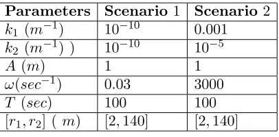
The parameters displayed in Table 1 are for two scenarios. The parameters in Scenario 1 are used in the simulation to estimatei1and reciprocally Scenario 2 for i2. As previously mentioned in the definition of the energy spaces (e.g,Definition 3), the energy function is said ”associate” with the energy space. In other words, one can estimate the energy of∂i
tΨ +,t
1 (f)(r0, t) and∂irΨ +,r
1 (f)(r, t0) for the various values ofi inZ+− {0}. Figure 1 and 2 displays the results. Note that the simula-tions are performed using Matlab (v9.0 R2016a-mathworks.com).
The top figures in Figure 1 and 2 correspond to the numerical estimation of the energy of the operators ∂i
tΨ +,t
1 (f)(r0, t) (also called ∂ti[[f]0] +,t
1 (r0, t))) and f ∂i
rΨ +,r
1 (f)(r, t0) (also called ∂ri[[f]0] +,r
1 (r, t0))). Thus, the results shows that for i > 2, the values of E(∂i
tΨ +,t
1 (f)(r0, t)) and E(∂irΨ +,r
Figure 1. Results from the estimation of the energy of ∂i
tΨ +,t
1 (f)(r0, t) and ∂ti[[f]1] +,t
1 (r0, t)). The Figures correspond to Scenario 1.
Figure 2. Results from the estimation of the energy of ∂i
rΨ +,r
1 (f)(r, t0) and∂ri[[f]1] +,r
Table 1. Parameters for the scenarios 1 and 2
Parameters Scenario
1
Scenario
2
k
1(
m
−1)
10
−100.001
k
2(
m
−1) )
10
−1010
−5A
(
m
)
1
1
ω
(
sec
−1)
0.03
3000
T
(
sec
)
100
100
[
r
1, r
2] (
m
)
[2
,
140]
[2
,
140]
Now, if we want to use the generalized energy operators (andTheorem2) with p inZ+andp >0, then one can look at solutions in the energy spaceEp(e.g, Section
2.2). It is the solutions of the kind ([[f]p]+,t
1 )n or ([[f]p] +,r
1 )n. Thus, the definition of the subspacesNi
1andNi2can be extend with pin Z+ such as
Ni1,p = {g∈S−(R2), ∀t∈[0, T], r0∈[r1, r2]|g(r0, t) =∂ i t([[f]
p
]+1,t) n
(r0, t), f ∈s−p(R
2), n∈
Z+− {0,1}}
Ni2,p = {g∈S−(R2),∀r∈[r1, r2], t0∈[0, T]|g(r, t0) =∂ i r([[f]
p
]+1,r) n
(r, t0), f ∈s−p(R
2), n∈
Z+− {0,1}}
With this definition, let us do a similar numerical estimation of the solutions and finding i1 and i2 for the case p = 1. The bottom figures of Figure 1 and 2 are the results. We can see that there is a factor of 10−4 and 10−11 in Scenario 1
and 2 respectively between the estimated energy for the operators corresponding to the case p= 0 and p= 1. Thus, one can conclude thati1 andi2 are equal to 0. Recalling the decompositionTheorem1 (and equation (3.3)), the energy space E0 is reduced to{0}.
4.3. Phenomenon of Duplication of Waves in a Closed Cavity. This section reflects on the idea of propagating electromagnetic waves in a closed cavity [2]. Here, the idea is not to revise the whole theory of electromagnetism, but rather discussing at a theoretical level the implication of our proposed model in this example and defining theduplication of waves.
in time overdt inside the cavity at a specific locationr0 (r0 in [r1, r2]) such as
E(f(r0, T)) =
Z T
0
(f(r0, u))2du <∞
E(f(r0, T +dt)) = E(f(r0, T)) +
∞ X
k=0 ∂k
t(f
2(r0, T))(dt)k k! <∞
E(f(r0, T +dt)) = E(f(r0, T)) +
∞ X
k=0 ∂k
t(f
2(r0, T))(dt)k k! <∞
E(f(r0, T +dt)) = E(f(r0, T)) +f2(r0, T)dt+
∞ X
k=1 ∂k−1
t Ψ
+,t
1 (f)(r0, T)
+Ψ−1,t(f)(r0, T)
(dt)
k+1
k+ 1! <∞
E(f(r0, T +dt)) ≃ E(f(r0, T)) +f2(r0, T)dt (4.8)
Note that by definition Ψ−1,t(f)(r0, T) = 0. Here the symbol ’≃’ means that
∃ ǫ∈R+, ǫ <<1, ∀k∈Z+, k >0| |∂kt−1 Ψ +,t
1 (f)(r0, T)
|< ǫ|f2(r0, T)| (4.9)
Now, let us do a hypothesis that E(f(r0, T +dt)) increases significantly over dt modifying the approximation in (4.9)
∃ ǫ∈R+, ǫ <<1, ∀k∈Z+, k >1| |∂kt−1Ψ +,t
1 (f)(r0, T)|< ǫ|Ψ +,t
1 (f)(r0, T)| (4.10) and then,
E(f(r0, T+dt)) ≃ E(f(r0, T)) +f2(r0, T)dt+ Ψ+1,t(f)(r0, T)dt 2
2
(4.11)
Now, using theTheorem1 and the model based on the energy space in the previous sections, one can say that the subspace N1
1 defined in Section 4.1 is not reduced to {0}. Thus, the solutions from this subspace has to be taken into account. The duplication of wave can be formulated as an approximation for taking into account additional solutions produced by the wave equation.
5. Conclusions
The core of this work is to define the notion of multiplicity of the solutions of a linear PDE using the model associated with energy spaces and the (generalized) energy operators. In this way, it contradicts the classical way of solving a nomi-nated PDE with boundaries conditions, but it rather focuses on additional solutions from these energy spaces. Themultiplicity is defined throughTheorem2 and the Corollary 1. The work shows how the energy operators (and generalized energy operators) can determine which energy subspace is reduced to{0}.
Furthermore, it was explained in Section 3.4 that the linearity of the PDEs does not play any role in Theorem 2 and the Corollary 1. As a matter of fact, the model with the energy subspace is applied directly to the form of the solutions of the nominated PDE (i.e. evanescent waves solution of the wave equation) with the conditions that the solutions are finite energy and in the Schwartz spaceS−(R2). Thus, there is no restriction theoretically speaking to use this model with non-linear PDEs. Our next interest is to apply our model to the type of solutions of the Korteweg de Vries equation called solitons which filled in the properties required to apply this model (e.g, finite energy function, solution in the Schwartz spaceS−(R2) ).
To conclude, the multiplicity of the solutions applied to the wave equation is only the first step before wondering if the receiving waves in a transmitter-receiver sys-tem, can be a sum of all those solutions. In other words, one can ask if the signal is generated by receiving not one type of solution/wave, but the additional solu-tions/waves coming from other energy subspaces.
Acknowledgments. The author wants to dedicate his work to vale Emeritus Prof. Alan G.R. McIntosh (FAA) former member of the center for mathematics and its applications in the school of mathematical sciences at the Australian National University. He kindly introduced me to the Schwartz space theory when many years ago I started the development of the mathematical frame on energy operators.
The authors would like also to thank the anonymous referee for his/her comments that helped us improve this article.
References
[1] E. Amzallag, J. Cipriani, N. Piccioli,Ondes, 1st Ed., Ediscience international, Paris, 1997. [2] G. Annino, H. Yashiro, M. Cassettari, M. Martinelli,Properties of trapped electromagnetic
modes in coupled waveguides, Phys. Rev. B 73, 125308, 2006.
[3] A. C. Bovik, J. P. Havlicek, and M. D. Desai, Theorems for Discrete Filtered Modulated Signals, in Proc. IEEE Int. Conference on Accoustics, Speech, and Signal Processing, 1993 (ICASSP-93), Vol.3, pp. 153-156., 27-30 April.
[4] K. Bryan, The Wave Equation II, lecture material, available at https://www.rose-hulman.edu/ bryan/lottamath/wave1.pdf
[5] J.C. Cexus, A.O. Boudraa, A. Baussard, F.H. Ardeyeh, E.H.S. Diop, 2D Cross-B-Energy Operator for images analysis, in proc. International Symposium on Communications, Control and Signal Processing (ISCCSP), pp. 1-4, 2010. doi: 10.1109/ISCCSP.2010.5463398 [6] R.B. Dunn, T.F. Quatieri, J.F. Kaiser,Detection of transient signals using the energy
op-erator, in Proc. IEEE Int. Conference on Acoustics, Speech, and Signal Processing, 1993 (ICASSP-93.), vol.3, pp.145-148, 27-30 April.
[7] G. H. Hardy, J. E. Littlewood, G. Plya,Inequalities, Cambridge Mathematical Library, 1988. [8] J. K. Hunter,Introduction to real analysis, University of California at Davis. 2012, available
athttps://www.math.ucdavis.edu/ hunter/m125a/introanalysisch7.pdf
[9] V. Kandia, Y. Stylianou,Detection of sperm whale clicks based on the Teager-Kaiser energy operator, International workshop on detection and localization of marine mammals using passive acoustics (No2), Monaco, 2006, vol. 67, pp. 1144-1163.
[10] J. F. Kaiser,On a simple algorithm to calculate the ’energy’ of a signal, in Proc. IEEE Int. Conference on Acoustics, Speech, and Signal Processing (ICASSP-90), vol. 1, pp. 381-384. [11] E. Kreizig,Advanced Engineering Mathematics, 8th Edition, John Wiley & Sons, 2003. [12] P. Maragos and A. Potamianos, Higher Order Differential Energy Operators, IEEE Signal
Processing Letters, vol. 2, No 8, 1995, pp 152-154.
[14] J.P. Montillet, The Generalization of the Decomposition of Functions by Energy Opera-tors, Acta Applicandae Mathematicae. doi: 10.1007/s10440-013-9829-0 (or also available in: http://arxiv.org/abs/1208.3385).
[15] J.P. Montillet,The Generalization of the Decomposition of Functions by Energy Operators (Part II) and Some Applications, Acta Applicandae Mathematicae. doi: 10.1007/s10440-014-9978-9 (or also available in: http://arxiv.org/abs/1308.0874).
[16] R. Petit,Ondes Electromagnetiques en radioelectricite et en optique, 2nd Edition, Masson, 1993.
[17] F. Salzenstein, P. Montgomery, and A. O. Boudraa,Local frequency and envelope estimation by Teager-Kaiser energy operators in white-light scanning interferometry, Optics Express, Vol. 22 (15), pp. 18325-18334, 2014. doi: 10.1364/OE.22.018325
[18] A. Schasse, R. Martin,Localization of Acoustic Sources Based on the Teager-Kaiser Energy Operator, in Proc. 18th European Signal Processing Conference (EUSIPCO-2010), Aalborg, Denmark, August 23-27, 2010.
AppendixA. Discussion aboutn in Z
Here is the discussion written in [15] (Section 4) in the case of the generalized energy operators about extending Theorem 1 and Lemma 1 with n in Z. The extension of Theorem 0 and Lemma 0 can be found in [14] (Section 3, p. 74). Let us recall:
Discussionn <−1: In this case, one can define:
∀f ∈S−p(R), ∀t∈R, p∈Z+, ([[f(t)]p]+1
n
6
= 0, ∀n∈Z+, n >1, 1 [[f(t)]p]+
1
n
(A.1) This set of functions can also be described as: finS−
p(R) andfnot inKer [[f(t)]p]+1
forpin Z+. Note that one could also chose to have f in s−
p(R). However, this is
more restrictive than the set defined in (A.1). Using an intermediary function, h such ash= 1
[[f(t)]p]+ 1
, the problem of decomposing∂k
t [[f(t)]p] + 1
−n
(kinZ+− {0}) is equivalent to resolving∂k
thn, which has been demonstrated in theLemma1 and Theorem1.
Discussionn= 1 orn=−1: As already underlined in [14], one can use a general formula forf in the set defined in equation (A.1):
∂tk [[f(t)] p
]+1
= ∂tk
[[f(t)]p]+ 1
3
[[f(t)]p]+ 1
2
k= 1, ∂t [[f(t)]p]+1
= [[f(t)]p]+1
−2
∂t [[f(t)]p]+1
3
+ [[f(t)]p]+1
3
∂t [[f(t)]p]+1
−2
k= 2, ∂t2 [[f(t)] p
]+1
= 2∂t [[f(t)]p]+1
−2
∂t [[f(t)]p]+1
3
+ [[f(t)]p]+1
3
∂2t [[f(t)] p
]+1
−2
+ [[f(t)]p]+1
−2
∂t2 [[f(t)] p
]+1
3
(A.2)
The example fork={1,2}in Equation (A.2) shows that∂k
t [[f(t)]p] + 1
can be de-composed into a product of successive derivatives of [[f(t)]p]+
1
3
and [[f(t)]p]+ 1
−2
Now for the casen=−1, it is easy to see that :
∂k t [[f(t)]
p]+ 1
−1
= ∂k t
[[f(t)]p]+ 1
2
[[f(t)]p]+ 1
3
(A.3)
With the discussion for the case n = 1, we can conclude that ∂k
t [[f(t)]p] + 1
−1
can be decomposed into a product of successive derivatives of [[f(t)]p]+ 1
2
and [[f(t)]p]+
1
−3
.
Jean-Philippe Montillet
ESPlab, STI IMT, Ecole Polytechnique de Lausanne, MC A3 301 (Microcity), Rue de la Maladire 71b, CH-2002 Neuchtel, Switzerland
![Figure 1.Results from the estimation of the energy of∂itΨ+,t1 (f)(r0, t) and ∂it[[f]1]+,t1(r0, t))](https://thumb-us.123doks.com/thumbv2/123dok_us/8762434.1752698/12.612.169.563.460.662/figure-results-estimation-energy-itps-t-f-r.webp)