Robust Backstepping Sliding Mode Control with L2-Gain Performance for Reference Input Wheel Slip Tracking of Vehicle

(1)

The wheel slip control is the basis of active safety control systems and intelligent driver assistance systems. This paper presents a new robust backstepping sliding mode controller for reference input wheel slip tracking based on the single-corner model combined with the actuator dynamics. The proposed controller is realized by combining backstepping method, which has the merits of simplified and flexible design procedure, with sliding mode control, which has robustness against system uncertainty and external disturbance. Moreover, the closed-loop wheel dynamic system is L2-gain stable by Lyapunov-based method, and the simulation results show that the proposed controller has better performance.

KEYWORDS: Wheel slip control, Backstepping method, Sliding mode control, L2-gain stable, Robustness.

Robust Backstepping Sliding Mode

Control with

L

₂

-Gain Performance

for Reference Input Wheel Slip

Tracking of Vehicle

ITC 4/48 Information Technology and Control

Vol. 48 / No. 4 / 2019 pp. 660-672

DOI 10.5755/j01.itc.48.4.24297

Robust Backstepping Sliding Mode Control with L2-Gain Performance for

Reference Input Wheel Slip Tracking of Vehicle

Received 2018/07/08 Accepted after revision 2019/09/27

http://dx.doi.org/10.5755/j01.itc.48.4.24297

Corresponding author: [email protected]

Jiaxu Zhang

State key Laboratory of Automotive Simulation and Control, Jilin University, Changchun 130022, China; Research and Development Center, China FAW Group Corporation, Changchun 130022, China;

e-mail: [email protected]

Jing Li

State key Laboratory of Automotive Simulation and Control, Jilin University, Changchun 130022, China; e-mail: [email protected]

1. Introduction

Active safety control systems and intelligent driver

(2)

especially in traffic jams or long-distance driving cir-cumstances. However, the wheel slip control is the basis of active safety control systems and intelligent driver assistance systems. For instance, the anti-lock brake system (ABS) regulates the slip of each wheel at its optimum value to prevent it from locking during braking, such that the shortest stopping distance is achieved and the capability of directional stability and steer-handling is maintained [4]. The electronic stability program (ESP) may produce additional yaw moment by commanding the target slip of one or two wheels to prevent vehicle from spinning and drifting out of lane [29]. Finally, the adaptive cruise control system (ACC) can follow target speed or forward ve-hicle at the desired safety headway distance by com-manding the target slip of the wheels and the target torque of the power system [16]. As a consequence, de-signing the wheel slip controller has important theo-retical and practical significance for active safety con-trol systems and intelligent driver assistance systems. In recent years, many control approaches which are robust against system uncertainty and external dis-turbance have been proposed for the wheel slip con-trol due to the modeling errors, the measurement or estimation errors, and the changing of external en-vironment conditions of the wheel dynamic system, such as sliding mode control [23], hybrid control [25] and fuzzy control [13], etc. Johansen et al. [9] established the speed-dependent nominal linearized slip model with a perturbation term as a basis for the wheel slip control, and utilized gain-scheduled LQR approach to design the gain matrices of the control-ler. Pasillas-Lépine [19] adopted wheel deceleration logic-based switching and wheel dynamic model to design the five-phase anti-lock brake algorithm, and proved the existence and stability of limit cycles by the Poincaré map. Hsu [7] proposed an intelligent exponential sliding-mode control strategy for ABS, and a functional recurrent fuzzy neural network uncertainty estimator was designed to reduce the chattering of the exponential sliding-mode control strategy by approximating and compensating the unknown nolinear term of ABS dynamics on-line. Jing et al. [8] presented a switched control strategy for the anti-lock brake system and then analyzed the stability condition of the closed-loop system by Lyapunov-based method in the Filippov frame-work. The proposed control strategy in [7-9, 19] may

(3)

conjunction with radial basis function neural net-work (RBFNN), which was used to improve the ro-bustness of the system by estimating the unknown uncertainties of the system on-line. Sardarmehni et al. [20] proposed two model-free wheel slip control-ler on the basis of fuzzy logic control approach and neural predictive control aproach, and simulation results showed that the neural predictive control approach had more robustness against exogenous disturbances and modeling uncertainties. In [2, 12, 15, 20], the uncertainty observer improves the ro-bustness of the system, but increases the complexity of the system. Therefore, it is absolutely essential to design the wheel slip controller which has both ro-bustness against system uncertainty and external disturbance and simple system structure.

The standard backstepping method introduced in [5, 17] provides a recursive Lyapunov-based frame-work for the controller design of the lower-triangu-lar nonlinear system and has the merits of simplified and flexible design procedure. However, the stan-dard backstepping method is not robust against the system uncertainty and external disturbance. This paper surmounts the demerit of the standard stepping method by combining the standard back-stepping method with sliding mode control which is insensitive to system uncertainty and external dis-turbance, and a backstepping sliding mode design framework is proposed. Compared with the nonlin-ear L2-gain control method [28], the backstepping sliding mode design framework can avoid solving the complex Hamilton-Jacobi-Issacs inequality to attain the same control objective that the ratio of the

L2 norm of the system output to the L2 norm of the lumped disturbance is less than the given threshold value. Then, a new robust backstepping sliding mode controller (RBSMC) with L2-gain performance for reference input wheel slip tracking is derived based on a single-corner vehicle model with actuator dy-namics and the backstepping sliding mode design framework. Moreover, the effectiveness of the pro-posed controller is verified based on vehicle dynam-ics simulation software.

This paper is organized as follows. Section 2 provides the dynamic model. Section 3 shows the nonlinear ro-bust controller. Section 4 introduces our simulations and results. Finally, Section 5 draws the main conclu-sion of our work.

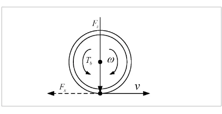
Figure 1

The single-corner model

2. System Modelling

The proposed RBSMC for reference input wheel slip tracking is based on a single-corner model, as it pro-vides a simple yet sufficiently rich description of the braking dynamics. As shown in Figure 1, the degrees of freedom for the model consists of the vehicle speed and the angular speed of the wheel.

In order to simplify the nonlinear controller design, the following modeling assumptions are made: 1 the vehicle is moving on a flat horizontal plane; 2 the suspension dynamics are neglected; 3 the wheel radius is assumed to be constant; 4 the tire camber and the tire sideslip angle are

as-sumed to be zero;

5 the tire relaxation dynamics are neglected. The single-corner model is given by [21]

x b

Jω = rF T− ₍₁₎

x

mv= −F, ₍₂₎

where ω is the angular speed of the wheel; v is the ve-hicle speed; Tb is the braking torque; Fx is the longitu-dinal tire-road contact force; J, m and r are the wheel inertia, the single-corner mass and the effective roll-ing wheel radius, respectively.

The wheel slip λ is defined by

v r

v ω

λ= − . ₍₃₎

(4)

[3] has been used to describe the nonlinear relation-ship of the tire-road friction coefficient and the wheel slip, as it is simple and has a good degree of accuracy:

( )

(

2

)

1 1 r 3

r e λϑ r

µ λ ₌ϑ ₋ − ₋λϑ _,

(4)

where ϑ_r₁ is the maximum value of friction curve; ϑr2

is the friction curve shape; ϑ_r₃ is the friction curve dif-ference between the maximum value and the value at

1

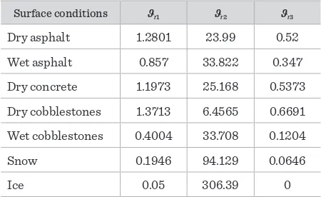
λ= . By changing the values of these three parame-ters, many different tire-road friction conditions can be modeled. The parameters of Burckhardt model for different road surfaces are listed in Table 1 [10].

The longitudinal tire-road contact force is expressed as

( )

x z

F =Fµ λ , (5)

where Fz is the vertical force at the tire-road contact point.

The derivative of Eq. (3) with respect to time yields

(

)

1 1 v r

v

λ= _ −λ _−ω_ __. ₍₆₎

Substituting Eqs. (1), (2) and (5) into Eq. (6) yields

2

1 1 _{( )}

z b

r _F r _T

v m J Jv

λ

λ= − _ − + _ µ λ +

 

 _. ₍₇₎

Time delays may cause instability and performance deterioration of system [30]. Taking brake lag into ac-count, the actuator dynamics [27] is given by

1 1

b b

T u

s

τ

=

+ , (8)

where τb is dimensionless time constant; u is the ac-tual control input.

The derivate of Eq. (8) with respect to time yields

1 1

b b

T = −_τ T +_τ u_. ₍₉₎

Since the vehicle speed dynamics are much slower than the wheel slip dynamics due to large differenc-es in inertia, the vehicle speed

v

can be regarded as a slowly-varying parameter. Hence, the Eq. (2) can be neglected, and we consider only the wheel slip dynamics with the actuator dynamics. Furthermore, we define the state variables x₁=λ λ− d, x T2= b, where

d

λ is the reference input wheel slip. Eqs.(7) and (9) are merged together into the state-space form of the nominal model as follows

(

)

2 1

1 1 2

2 2

1

1 ₍ ₎

1

d

z d

b

x r r

x F x x

v m J Jv

x x u

λ _µ _λ

τ

 _{= −}  − − ₊  ₊ ₊

  

  



 = − −





. (10)

Consider the nominal model with the lumped uncer-tainty, Eq.(10) can be rewritten as

( )

(

)

1 1 2 1

1

2 2 2

: 1

b

x f x Gx d

x x u d

ψ

τ

= + +

 

 = − − +





 , (11)

where

( )

1 2

1 1 1 x d r z ( 1 d)

f x F x

v m J

λ _µ _λ

 − − 

= − _ + _ +

  ,

r G

Jv = and

[

]

T

1 2

d= d d _{is the lumped uncertainty that contains}

system uncertainty and external disturbance.

3. Robust Backstepping Sliding

Mode Controller Design

In this section, sliding mode control combined with backstepping method is used to derive the RBSMC for reference input wheel slip tracking, which integrates Table 1

Parameters of Burckhardt model for different road surfaces

Surface conditions ϑr1 ϑr2 ϑr3

Dry asphalt 1.2801 23.99 0.52

Wet asphalt 0.857 33.822 0.347

Dry concrete 1.1973 25.168 0.5373

Dry cobblestones 1.3713 6.4565 0.6691

Wet cobblestones 0.4004 33.708 0.1204

Snow 0.1946 94.129 0.0646

(5)

both the merits of sliding mode control and backs-tepping method. Based on the standard backsbacks-tepping method, we employ the change of coordinates

1 1

2 2 1

z x

z x α

= 

 = −

 , (12)

where α1 is virtual controller.

Define the output of the system ψ₁

[

]

T 1 1 2 2

z= κ z κ z ,

where κ₁ and κ₂ are nonnegative weight coefficients, and the system ψ₁ is rewritten

( )

(

)

[

]

1 1 2 1

2 2 2 2

T 1 1 2 2

1 :

b

x f x Gx d

x x u d

z z z

ψ τ κ κ  = + +   = − − +    =  

 . ₍₁₃₎

The aim of this paper is to design a RBSMC for the system ψ₂ such that the closed-loop wheel dynamic system is asymptotically stable when the disturbance

0

d = , and is L2-gain stable when the disturbance d ≠0, which means that the relationship of the output of the system ψ₂ and the disturbance satisfies the following inequality

T 2 2 T 2

0 z dt≤γ 0 d dt

∫

(14)

for all T ≥0 and all d L∈ 2

(

0,T

)

, where γ is positive

constant.

The design procedure is elaborated in the following steps.

Step 1: Define the first storage function 2 1 1₂ 1

V = z . Note that

( )

(

)

1 1 1 2 1

1 2 1 1

z x f x Gx d

f x G z α d

= = + + = + + +  

( )

(

)

1 1 1 2 1

1 2 1 1

z x f x Gx d

f x G z α d

= = + + = + + +   . (15)

Differentiating the first storage function V₁ along the trajectories of the system ψ2 and substituting Eq. (15)

into it, it is easy to have

( )

(

)

(

)

1 1 1 1 1 2 1 1

V =z z_ =z f x +G z +α +d _. ₍₁₆₎

By viewing x₂ as a virtual control input, let us choose virtual controller α1 as follows

( )

(

)

1

1 G c z1 1 f x1

α _{= −} − ₊ _,

(17)

where c1 is positive constant, and then

(

)

1 1 1 1 2 1

V =z −c z Gz d+ + _. ₍₁₈₎

Define the function

(

)

(

)

(

)

2 ₂ 2

1 1 1

1 1 1 2 1

2 2 2 2 2 2

1 1 2 2 1

1 2

H V z d

z c z Gz d

z z d

γ κ κ γ = + − = − + + + + −  . ₍₁₉₎

Step 2: Define the sliding surface σ=c z z_{0 1}+ ₂, where 0

c is the design parameter. Note that

(

)

2 2 1 1 2 2 1

b

z x α x u d α

τ

=  −  = − − + − 

 , ₍₂₀₎

where

( )

( ) (

)

1 1

1 1 1 1

1 1 1

1 1 1 2 1

1

f x

G c z x

x f x

G c c z Gz d

x α − − ∂   = − _ + _ ∂   ∂   = − _ + _ − + + ∂      (21)

( )

2 1 1 1 1 1 1

1 ( )

1

1 ₍ ₎

d d

z

z d

x _{r F} x

f x m J x

x v F x m λ µ λ µ λ  − − ₊  ∂ +     ∂ _{= −} __ _ ∂ _   ∂ − +     . (22)

Differentiating the sliding surface σ and substituting Eqs. (15) and (20) into it, it is easy to have









0 1 2 0 1 1 2 1

2 2 1

1 b

c z z c c z Gz d

x u d

               

 . (23)

Augment the storage function of Step 1, and thus the new storage function is given by

2 2 1 1₂

V V= + σ . (24)

(6)

(

2 2 2

)

2 2 1₂

H =V + z −γ d _. ₍₂₅₎

Substituting Eq. (19) into Eq. (25) yields









_

_

















  



2 2 2

2 1 1 2 22

1 1 1 2 1 2 2 2 2 2 2 2 2

1 1 2 2 1

2 1 1 1 2 1 2 2 2 2 2 2 2 2

1 1 2 2 1 2

0 1 1 2 1 2 2

1 1

1 1 1 2 1

1 1 2 1 2 1 1 2 2 1 2 1 b

H V z d H d

z c z Gz d z z d

d z c z Gz d

z z d d

c c z Gz d x u d

f x

G c c z Gz d

x                                          _ _ _ _ _{ }        _ _ _           _ _ _     _   (26)

Choose the actual controller as









 

_{ }

1 2

1 0 1 1 1 0 0 1 0 2

0

1 1

1

1 1 2

1 1

2 1

1 2 2 1 2

1

sgn ,

b b b

b b

b

u c c G c z c c G c G c z

c

f x f x

c G z z

x x

f x

c h h

x G                               _  _      (27)

where h₁ and h₂ are positive constants, and sgn

( )

σ de-notes signum function.

Substituting the actual controller expressed by Eq. (27) into Eq. (26), we can obtain





 

_{ }





2

2 1 1 1 2 1 1 1 12 2 2 22 2 2 21 2 22

1 1

2 0 1 2 1 1

0 1

2

1 1 2

1 2 2

1

2 2 2

1 1 2 0 1 1 0 1 2

0

2 2 2 2 2

0 2 1

2 2 1 1 2 2

1 2 sgn 1 1 2 b b

H c z Gz z z d z z d d

f x

G z c d d G c d

c x

f x h h

c

x G

G

c z z c z d c z d

c c z d

z d z z

      _ _                            _             _ _ _ _     _              



 



 

_{ }

2 2 2

1 2 2 2 1 2 2 1 1 1 1 1 2 4

2 b b sgn .

d d

f x h

d d c x G h     _             _   _  _       (28)

By using Young’s inequality [1], we can obtain

(

2

)

(

02

)

2 2 2 2

0 1 1 2 1 1

2 1 ₁

1

8

c

c z d z γ d

γ

+

+ ≤ + (29)

2

2 2 2

0

0 1 2 2 1 2

1 4

c

c z d z γ d

γ

≤ + (30)

2

2 2 2

0

0 2 1 2 2 1

2 1

8

c

c z d z γ d

γ

≤ + (31)

2 2 2

2 2 2 2 2

1 1

4

z d z γ d

γ

≤ + . ₍₃₂₎

Substituting the inequalities (29), (30), (31) and (32) into Eq. (28) yields

(

)

( )

2

2 ₂ ₂

0 0 1 2

2 1 2 2 1

2 2 2 0 2 2 2 2 0 2 1 1 1 1 2 1 2 2 1 2 2 1 2 2 sgn b b c _c

H c z

c G _z c f x d c x G h h κ γ γ κ γ γ γ σ γ σ σ σ τ τ  ₊    ≤ − − − −       −_ − − − _     ∂   −_ − + _∂  _     − − . ₍₃₃₎

Choose the parameters c₀ and c₁ that satisfying the following inequalities

(

₂

)

2

2 2

0 ₀ ₁

1 2 2

2 1

0

2

c _c

c − _γ+ −_γ −κ > (34)

2 2

0 2

2 2

0

2 1 ₀

2 c G c κ γ γ

− − − > . (35)

Substituting the inequalities (34) and (35) into in-equality (33), we can obtain

2 0

H ≤ . (36)

Defining V x

( )

=V x2

( )

, and on the basis of Eq. (25)

and inequality (36), we can obtain

(

2 2 2

)

1 2

(7)

By the inequality (37), we can obtain the following in-equality when the disturbance d =0

2

1 2

V≤ − z _. ₍₃₈₎

Integrating both sides of the inequality (38), we can obtain

( )

(

)

(

( )

)

(

)

2

0 z dt 2 V x 0 V x ∞

≤ − ∞

∫

. (39)

Since V x

(

( )

0

)

is bounded and V x t

(

( )

)

is a positive, non-increasing function, we can obtain z L∈ 2. In

ad-dition, z, α₁, α₁, f x

( )

₁ , d₁, d₂∈L_∞, and we can get z L∈ ∞ using Eqs. (15) and (20). With z L∈ ₂L∞ and z L∈ ∞, we can get

( )

0 0

lim_t z t

→ = based on Barbalat’s lemma [26]. That implies that the closed-loop wheel dynamic system is asymptotically stable when the disturbance

0

d = .

Integrating both sides of the inequality (37), we can obtain the following dissipative inequality when the disturbance d ≠0

( )

(

)

(

( )

)

T

(

2 2 2

)

0

1

0

2

V x T −V x ≤

_∫

γ d − z dt_. (40)

Therefore, the closed-loop wheel dynamic system with respect to the supply rate

( )

_, 1

(

2 2 2

)

2

w d z = γ d − z is

dissipative, and according to the relationship be-tween the dissipativity of the system and the L2-gain stability of the system [22], the closed-loop wheel dy-namic system is also L2-gain stable.

Remark 1: It is easy to choose the parameters c0 and

1

c to satisfy the inequalities (34) and (35), due to the relationship of the parameters c0 and c1 is decoupled.

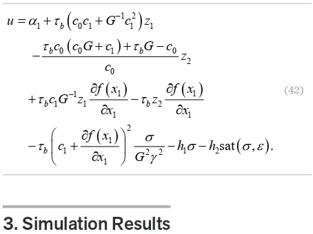
Remark 2: To eliminate the chattering phenomenon due to the actual control input containing the discon-tinuous signum function, the subsequent condiscon-tinuous saturation function is employed to replace the dis-continuous term [11]

(

)

( )

sat , sgn if if σ _{σ ε} σ ε ε σ σ ε  _<  =   _≥  , (41)

where ε>0 is the width of the boundary layer. Thus, the actual controller in Eq. (27) is rewritten

(

)

(

)

( )

₍

₎

1 2

1 0 1 1 1

0 0 1 0

2

0

1 1

1

1 1 2

1 1

2 1

1 2 2 1 2

1

sat , .

b

b b

b

u c c G c z

c c G c G c z c

f x f x

c G z z

x x

f x

c h h

x G α τ τ τ τ τ σ τ σ σ ε γ − − = + + + + − − ∂ ∂ + − ∂ ∂ ∂   − _ + _ − − ∂   (42)

3. Simulation Results

The performance of the proposed RBSMC for reference input wheel slip tracking has been verified by a full-ve-hicle dynamics simulation model (MSC CarSim®) with the actuator dynamics. MSC CarSim® is a comprehen-sive model for the efficient simulation of the whole vehicle dynamics, and it includes powertrain model, suspension model, aerodynamic model, and tire model with dynamic rolling resistance and relaxation length, etc. Therefore, the following simulation results can be considered very close to real-vehicle experiments. Straight line braking manoeuvres on a flat dry asphalt road (µ=1) and a flat wet asphalt road (µ=0.6) are performed for testing the performance of the proposed RBSMC. All parameters of the proposed RBSMC are set by κ₁=10, κ₂=0.01, c₀ =1, c₁=350, γ =50, h₁=3.2,

2 6

h = and ε=1. The main parameters of the full-vehi-cle dynamics simulation model are set by m=354kg,

2

0.9kg m

J = ⋅ and r=0.31m.

(8)

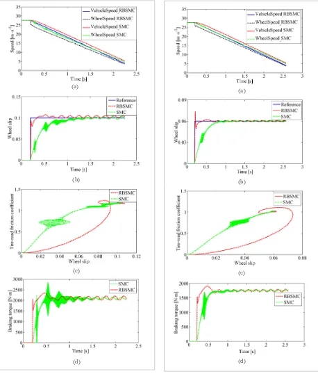
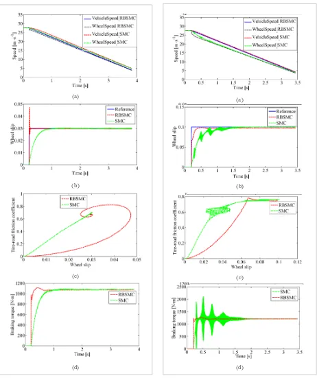
Figure 2

The simulation results of straight line braking manoeuvre on dry asphalt road surface with λd = 0.1: (a) vehicle speed

and wheel speed, (b) reference input wheel slip and actual wheel slip, (c) tire-road friction coefficient versus wheel slip, and (d) braking torque

(d) (d)

(c) _(c)

(b) _(b)

(a)

(a) Figure 3

The simulation results of straight line braking manoeuvre on dry asphalt road surface with λd = 0.06: (a) vehicle speed

(9)

Figure 4

The simulation results of straight line braking manoeuvre on dry asphalt road surface with λd = 0.03:

(a) vehicle speed and wheel speed, (b) reference input wheel slip and actual wheel slip, (c) tire-road friction coefficient versus wheel slip, and (d) braking torque

Figure 5

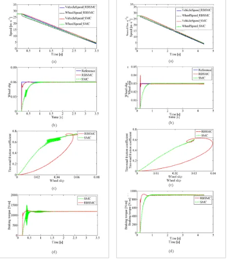
The simulation results of straight line braking manoeuvre on wet asphalt road surface with λd = 0.1: (a) vehicle speed

(a) (a)

(d) (d)

(c) _(c)

(10)

Figure 6

Figure 7

(a) (a)

(d) (d)

(c) (c)

(11)

of RBSMC have faster dynamic response and better tracking precision than those of SMC in the transient state. That explains why the vehicle speeds and wheel speeds of RBSMC are smaller than those of SMC at the same time respectively. Figure 2(c), Figure 3(c) and Figure 4(c) show that the wheel slips of RBSMC have similar performance with those of SMC in the steady state. As shown in Figure 2(d), Figure 3(d) and Figure 4(d), the braking torques of RBSMC are more smoother than those of SMC. Moreover, in order to quantitatively evaluate the performance of the RB-SMC, the root mean-squared error (RMSE) between the reference input wheel slip and the actual value is computed. According to the statistical results shown as Table 2, the maximum RMSE of the proposed RB-SMC in the straight line braking manoeuvre on a flat dry asphalt road is 0.0059, while the maximum RMSE of SMC is 0.0219.

Table 2

Root mean-square error between the reference input wheel slip and actual value

Manoeuvre Reference RMSE

RBSMC SMC

Straight line braking on dry asphalt road

0.1 0.0059 0.0219

0.06 0.0025 0.0118

0.03 0.0011 0.0047

Straight line braking on wet asphalt road

0.1 0.0064 0.0176

0.06 0.0025 0.0099

0.03 0.0010 0.0043

compared with straight line braking manoeuvre on a flat dry asphalt road. Both RBSMC and SMC have great robustness against the system uncertainty and external disturbance, but the proposed RBSMC has better performance in the transient state. According to the statistical results shown as Table 2, the maxi-mum RMSE of the proposed RBSMC in the straight line braking manoeuvre on a flat wet asphalt road is 0.0064, while the maximum RMSE of SMC is 0.0176.

4. Simulation Results

This paper has presented a new robust backstepping sliding mode controller (RBSMC) for reference input wheel slip tracking based on the single-corner model with the actuator dynamics. The proposed RBSMC combines the merit of backstepping method that has simplified and flexible design procedure with the mer-it of sliding mode control that is insensmer-itive to system uncertainty and external disturbance, and the Lya-punov-based method is used to derive that the closed-loop wheel dynamic system is L2-gain stable. Then, the simulation based on the full-vehicle dynamics simulation model is implemented to validate the per-formance of the proposed RBSMC. The simulation results indicate that it can guarantee that the wheel slip follow the trend of the reference input quickly and accurately compared with the traditional sliding mode controller for reference input wheel slip tracking. In future works, the proposed RBSMC will be further tested and fine tuned on a real test vehicle equipped with by-wire electro-mechanical-brakes. Moreover, active safety control systems and intelligent driver assistance systems based on the proposed RBSMC should be researched.

Acknowledgement

This work is supported by National Key Research and Development Program of China (Grant No. 2016YFB0101002).

Second, straight line braking manoeuvre on a flat wet asphalt road is implemented with setting the initial vehicle speed 27.78m/s (equivalently 100km/h) and the desired wheel slip 0.1, 0.06, and 0.03, respectively, and Figures 5-7 show the simulation results for com-paring the performance of the proposed RBSMC with those of SMC. The similar results can be obtained

References

1. Alzer, H., Fonseca, C. M. D., Kovacec, A. Young-type Inequalities and Their Matrix Analogues. Linear and Multilinear Algebra, 2015, 63(3), 622-635. https://doi. org/10.1080/03081087.2014.891588

(12)

3. Burckhardt, M. Fahrwerktechnik: Radschlupf-Regel-systeme. Vogel Verlag, Würzburg, 1993.

4. Choi, S. B. Antilock Brake System with a Continuous Wheel Slip Control to Maximize the Braking Perfor-mance and the Ride Quality. IEEE Transactions on Control Systems Technology, 2008, 16(5), 996-1003. https://doi.org/10.1109/TCST.2007.916308

5. Das, A., Lewis, F., Subbarao, K. Backstepping Approach for Controlling a Quadrotor Using Lagrange Form Dy-namics. Journal of Intelligent & Robotic Systems, 2009, 56(1), 127-151. https://doi.org/10.1007/s10846-009-9331-0

6. Harifi, A., Aghagolzadeh, A., Alizadeh, G., Sadeghi, M. Designing a Sliding Mode Controller for Slip Control of Antilock Brake Systems. Transportation Research Part C, 2008, 16, 731-741. https://doi.org/10.1016/j. trc.2008.02.003

7. Hsu, C. F. Intelligent Exponential Sliding-Mode Control with Uncertainty Estimator for Antilock Braking Sys-tems. Neural Computing and Applications, 2016, 27(6), 1463-1475. https://doi.org/10.1007/s00521-015-1946-4 8. Jing, H. H., Liu, Z. Y., Chen, H. A Switched Control

Strategy for Antilock Braking System with on/off Valves. IEEE Transactions on Vehicular Technolo-gy, 2011, 60(4), 1470-1484. https://doi.org/10.1109/ TVT.2011.2125806

9. Johansen, T. A., Petersen, I., Kalkkuhl, J., Lüdemann, J. Gain-Scheduled Wheel Slip Control in Automotive Brake Systems. IEEE Transactions on Control Sys-tems Technology, 2003, 11(6), 799-811. https://doi. org/10.1109/TCST.2003.815607

10. Kiencke, U., Nielsen, L. Automotive Control Systems. Springer, Berlin, 2000.

11. Lee, D. Spacecraft Coupled Tracking Maneuver Using Sliding Mode Control with Input Saturation. Journal of Aerospace Engineering, 2015, 28(5), 401-413. https:// doi.org/10.1061/(ASCE)AS.1943-5525.0000473 12. Lin, C. M., Hsu, C. F. Neural-Network Hybrid Control

for Antilock Braking Systems. IEEE Transactions on Neural Networks, 2003, 14(2), 351-359. https://doi. org/10.1109/TNN.2002.806950

13. Mirzaei, A., Moallem, M., Dehkordi, B. M., Fahimi, B. Design of an Optimal Fuzzy Controller for Antilock Bra-king Systems. IEEE Transactions on Vehicular Tech-nology, 2006, 55(6), 1725-1730. https://doi.org/10.1109/ TVT.2006.878714

14. Mirzaei, M., Mirzaeinejad, H. Optimal Design of a Non-linear Controller for Anti-lock Braking

Sys-tem. Transportation Research Part C, 2012, 24, 19-35. https://doi.org/10.1016/j.trc.2012.01.008

15. Mirzaeinejad, H. Robust Predictive Control of Whe-el Slip in Antilock Braking Systems Based on Radial Basis Function Neural Network. Applied Soft Com-puting, 2018, 70, 318-329. https://doi.org/10.1016/j. asoc.2018.05.043

16. Moon, S., Moon, I., Yi, K. Design, Tuning, and Evaluati-on of a Full-range Adaptive Cruise CEvaluati-ontrol System with Collision Avoidance. Control Engineering Practice, 2009, 17(4), 442-455. https://doi.org/10.1016/j.coneng-prac.2008.09.006

17. Park, J. H. Synchronization of Genesio Chaotic System via Backstepping Approach. Chaos, Solitons & Fractals, 2006, 27(5), 1369-1375. https://doi.org/10.1016/j.cha-os.2005.05.001

18. Park, K. S., Lim, J. T. Wheel Slip Control for ABS with Time Delay Input using Feedback Linearization and Adaptive Sliding Mode Control. International Con-ference on Control, Automation and Systems, Seoul, Korea, 2008, 290-295. https://doi.org/10.1109/IC-CAS.2008.4694658

19. Pasillas-Lépine, W. Hybrid Modelling and Limit Cy-cle Analysis for a Class of Five-phase ABS Algorithms. Vehicle System Dynamics, 2006, 44(2), 173-188. https:// doi.org/10.1080/00423110500385873

20. Sardarmehni, T., Rahmani, H., Menhaj, M. B. Robust Control of Wheel Slip in Anti-lock Brake System of Au-tomobiles. Nonlinear Dynamics, 2014, 76(1), 125-138. https://doi.org/10.1007/s11071-013-1115-1

21. Savaresi, S. M., Tanelli, M. Active Braking Control Systems Design for Vehicles. Springer, London, 2010. https://doi.org/10.1007/978-1-84996-350-3

22. Schaft, A. V. D. L2-gain and Passivity Techniques in Nonlinear Control. Springer, Berlin, 1996. https://doi. org/10.1007/3-540-76074-1

23. Shim, T., Chang, S., Lee, S. Investigation of Sliding-Sur-face Design on the Performance of Sliding Mode Con-troller in Antilock Braking Systems. IEEE Transactions on Vehicular Technology, 2008, 57(2), 747-759. https:// doi.org/10.1109/TVT.2007.905391

24. Tanelli, M., Astolfi, A., Savaresi, S. M. Robust Nonline-ar Output Feedback Control for Brake by Wire Control Systems. Automatica, 2008, 44, 1078-1087. https://doi. org/10.1016/j.automatica.2007.08.020

(13)

International Journal of Vehicle Design, 2009, 82(4), 659-678. https://doi.org/10.1080/00207170802203598 26. Tao, G. A Simple Alternative to the Barbalat Lemma.

IEEE Transations on Automatic Control, 1997, 42(5), 698. https://doi.org/10.1109/9.580878

27. Yu, H. X., Qi, Z. Q., Duan, J. M., Taheri, S., Ma, Y. F. Multiple Model Adaptive Backstepping Control for Antilock Braking System based on LuGre Dynamic Tyre Model. International Journal of Vehicle Design, 2015, 69(1/2/3/4), 168-184. https://doi.org/10.1504/ IJVD.2015.073120

28. Zhao, J., Hill, D. J. On Stability, L2-gain and H∞ Control

for Switched Systems. Automatica, 2008, 44(5), 1220-1232.

29. Zhou, H. L., Liu, Z. Y. Vehicle Yaw Stability-Control Sys-tem Design based on Sliding Mode and Backstepping Control Approach. IEEE Transactions on Vehicu-lar Technology, 2010, 59(7), 3674-3678. https://doi. org/10.1109/TVT.2010.2050790