A COMPUTATIONAL SOFTWARE PROGRAM FOR DETERMINING THE COMBUSTION TEMPERATURES OF SOLID FUELS

60

A COMPUTATIONAL SOFTWARE PROGRAM FOR DETERMINING THE

COMBUSTION TEMPERATURES OF SOLID FUELS

Marta Kowalik1_{, Jarosław Boryca}1

1 _{The Department of Industrial Furnaces and Environmental Protection, The Faculty of Process & Material}

Engineering and Applied Physics, Technical University of Czestochowa, Al. Armii Krajowej 19, 42-200 Czestochowa, Poland, e-mail: [email protected]

INTRODUCTION

A basic combustion process control param-eter, aside from the excess air factor, is tempera-ture. The temperature of combustion is a factor determining the efficiency of heat transfer. Nor-mally, efforts are made to increase the combus -tion temperature with the aim of increasing the heat transfer efficiency. There are several meth -ods that allow the increase of this parameter, namely [1, 2]:

• heating up the fuel and incoming air,

• enriching the air with oxygen,

• thermal insulation of the combustion chamber,

• assuring the complete and total combustion with the lowest possible value of the excess air factor, α.

The proper selection of the combustion tem-perature allows the correctness of analytical, and in a particular model and design combustion pro-cess-related calculations, to be maintained. Deter-mining the combustion temperatures conditions, inter alia, model studies of the combustion of solid

fuels in the context of reducing atmospheric pollut-ant emissions. Hence, it seems to be of paramount importance to determine this parameter in an ef-ficient and, at the same time, expeditious manner.

COMBUSTION TEMPERATURE

The temperature that combustion gas attains at the end of the combustion process is called combustion temperature. Three combustion tem-perature types are distinguished [3–6].

The calorimetric combustion temperature is the highest temperature achievable by undissoci -ated combustion gas as a result of the adiabatic and isobaric combustion of fuel with theoretical amount of air [3, 5]:

1

sp r

kal

i

_c

i

t

=

0

+

₍₁₎

" s d

V

Q

i

₀

=

(2)

(

₉

)

₁₀

3

2500

10400

8

144030

33900

_

⋅











₊

_⋅

₋

₋











 −

⋅

+

⋅

=

c

h

o

s

w

h

Q

d c

(3)

" min

s

paliwa paliwa p

pow a

r

V

t

c

t

c

V

i

=

⋅

⋅

+

⋅

(4)

sp d r

teor

_c

i

i

i

t

=

α

+

−

₍₅₎

" s

d

V

Q

i

_α

=

(6)

O H O H CO

CO

d r r

i =12470⋅

α

₂ ⋅ ₂ +10620⋅

α

₂ ⋅ ₂

(7)

O H CO ,r

r _{2 2}

O H CO2,

α

2

α

teor

rzecz

t

t

=

µ

⋅

(8)

c

paliwa c h o n s p w

c =0.708⋅ +14.195⋅ +0.915⋅ +1.039⋅ +0.699⋅ +0.795⋅ +4.186⋅

∑

⋅ = ci r_i

c

(10)

2

t

C

t

B

A

c

i

=

+

⋅

+

⋅

(11)

3 1 2 1 1

1

B

t

C

t

D

t

A

+

⋅

+

⋅

+

⋅

=

α

( ) 2

{

(

2 ( ) 2

)

[

( ) 2 2

]

}

2 i 1 CO iCO i 1 CO i 1CO CO

CO

=

α

+

+

α

−

α

+

⋅

p

+

−

p

α

( )i HO

{

(

iHO ( )i HO

)

[

( )i HO HO

]

}

O

H2

=

α

+1 2

+

α

2

−

α

+1 2

⋅

p

+1 2

−

p

2

α

2

CO i

α

,

α

iH2O

( )i+1CO2

α

,

α

( )i+1 H2O

2

CO

p

,

pH2O

( )i 1CO2

p +

,

p( )i+1H2O

(1) where: c_sp – mean specific heat of combustion

gas, J/(μm3._K),

i₀ – enthalpy of 1 μm3 _{of wet theoretical} combustion gas (α = 1,0), J/μm3_, Research Journal

Volume 7, Issue 18, June 2013, pp. 60–67

DOI: 10.5604/20804075.1051258 Original Article

ABSTRACT

The combustion temperature is one of parameters influencing the efficiency of com-bustion process. The analytical, model and design calculations of processes related to fuel combustion and heat exchange intensity require the combustion temperature to be correctly determined. These are, however, complex, and, as a consequence, burdensome and time-consuming requirements. Developing an appropriate software program will considerably streamline the calculation procedure. Based on analytical relationships for the combustion process, a computational software program has been developed within this study, which enables the determination of the calorimetric, theo-retical and actual combustion temperatures of solid fuels.

Key words: combustion of solid fuels, combustion temperature, computational soft-ware program.

61

Advances in Science and Technology – Research Journal vol. 7 (18) 2013

i_r – combustion substrates enthalpy per 1 μm3 _{wet theoretical combustion gas, J/μm}3_. The enthalpy of wet theoretical combustion gas is expressed by the relationship [3, 5]:

" s d

V

Q

i

₀

=

₍₂₎

where: "

s

V

– unit of wet combustion gas volume, μm3

sp. wilg./kg fuel, Q_d – calorific value, J/kg:

1

sp r

kal

i

_c

i

t

=

0

+

₍₁₎

" s

d

V

Q

i

₀

=

(2)

(

₉

)

₁₀

3

2500

10400

8

144030

33900

_

⋅











−

−

⋅

+











 −

⋅

+

⋅

=

c

h

o

s

w

h

Q

_{d c}

(3)

" min s paliwa paliwa p pow a r

_V

t

c

t

c

V

i

=

⋅

⋅

+

⋅

(4)

sp d r

teor

i

_c

i

i

t

=

α

+

−

₍₅₎

" s

d

V

Q

i

_α

=

(6)

O H O H CO CO

d r r

i =12470⋅

α

₂ ⋅ ₂ +10620⋅

α

₂ ⋅ ₂

(7)

O H CO ,r

r _{2 2}

O H CO2,

α

2

α

teor

rzecz

t

t

=

µ

⋅

(8)

c

paliwa c h o n s p w

c =0.708⋅ +14.195⋅ +0.915⋅ +1.039⋅ +0.699⋅ +0.795⋅ +4.186⋅

∑

⋅ = ci r_i

c

(10)

2

t

C

t

B

A

ci

=

+

⋅

+

⋅

(11)

3 1 2 1 1

1

B

t

C

t

D

t

A

+

⋅

+

⋅

+

⋅

=

α

( ) 2

{

(

2 ( ) 2

)

[

( ) 2 2

]

}

2 i 1 CO iCO i 1 CO i 1CO CO

CO

=

α

+

+

α

−

α

+

⋅

p

+

−

p

α

( )i HO

{

(

iHO ( )i HO

)

[

( )i HO HO

]

}

O

H2

=

α

+1 2

+

α

2

−

α

+1 2

⋅

p

+1 2

−

p

2

α

2

CO i

α

,

α

iH2O

( )i+1CO2

α

,

α

( )i+1 H2O

2

CO

p

,

pH2O

( )i 1CO2

p +

,

p( )i+1H2O

(3)

where: c, s, h, o, w_c – mass fractions of liquid and solid fuel components.

The enthalpy of combustion substrates per 1 μm3 _{of theoretical wet combustion gas is determined}

from the relationship [3]:

" min s fuel fuel p pow a r

_V

t

c

t

c

V

i

=

⋅

⋅

+

⋅

(4)

where: c_pow – mean specific heat capacity of combustion air, J/(μm3._K), c_fuel – mean specific heat capacity of combustion gas, J/(kg ._K), t_p – combustion air temperature, °C,

t_fuel – fuel temperature, °C,

V_{a min} – minimum combustion air demand, μm3

pow./ kgfuel,

The theoretical (initial) combustion temperature is the highest temperature achievable by dissoci-ated combustion gas [3, 5]:

sp d r

teor

i

_c

i

i

t

=

a

+

(5)

where: i_α – enthalpy of 1 μm3 _{of wet real combustion gas allowing for the value of the excess air factor,}

J/μm3_,

i_d – enthalpy of dissociation of 1 μm3 _{of real combustion gas, J/μm}3_.

The enthalpy of wet real combustion gas, while allowing for the value of the excess air factor, is expressed by the relationship [3, 5]:

_"

s d

V

Q

i

_a

=

(6)

The enthalpy of real combustion gas dissociation is determined from the relationship:

sp r

kal

i

_c

i

t

=

0

+

₍₁₎

" s

d

V

Q

i

₀

=

(2)

(

₉

)

₁₀

3

2500

10400

8

144030

33900

_

⋅











−

−

⋅

+











 −

⋅

+

⋅

=

c

h

o

s

w

h

Q

d c

(3)

" min s paliwa paliwa p pow a r

_V

t

c

t

c

V

i

=

⋅

⋅

+

⋅

(4)

sp d r

teor

i

_c

i

i

t

=

α

+

−

₍₅₎

" s d

V

Q

i

_α

=

(6)

O H O H CO CO

d r r

i =12470⋅

α

₂ ⋅ ₂ +10620⋅

α

₂ ⋅ ₂

(7)

O H

CO ,r

r _{2 2}

O H CO2,

α

2

α

teor

rzecz

t

t

=

µ

⋅

(8)

c

paliwa c h o n s p w

c =0.708⋅ +14.195⋅ +0.915⋅ +1.039⋅ +0.699⋅ +0.795⋅ +4.186⋅

∑

⋅

= ci r_i

c

(10)

2

t

C

t

B

A

ci

=

+

⋅

+

⋅

(11)

3 1 2 1 1

1

B

t

C

t

D

t

A

+

⋅

+

⋅

+

⋅

=

α

( ) 2

{

(

2 ( ) 2

)

[

( ) 2 2

]

}

2 i 1 CO iCO i 1 CO i 1CO CO

CO

=

α

+

+

α

−

α

+

⋅

p

+

−

p

α

( )i HO

{

(

iHO ( )i HO

)

[

( )i HO HO

]

}

O

H2

=

α

+1 2

+

α

2

−

α

+1 2

⋅

p

+1 2

−

p

2

α

2

CO i

α

,

α

iH2O

( )i+1 CO2

α

,

α

( )i+1 H2O

2

CO

p

,

pH2O

( )i 1CO2

p +

,

p( )i+1H2O

(7) where:

sp r

kal

i

_c

i

t

=

0

+

₍₁₎

" s d

V

Q

i

₀

=

(2)

(

₉

)

₁₀

3

2500

10400

8

144030

33900

_

⋅











−

−

⋅

+











 −

⋅

+

⋅

=

c

h

o

s

w

h

Q

d c

(3)

" min s paliwa paliwa p pow a r

_V

t

c

t

c

V

i

=

⋅

⋅

+

⋅

(4)

sp d r

teor

i

_c

i

i

t

=

α

+

−

₍₅₎

" s

d

V

Q

i

_α

=

(6)

O H O H CO CO

d r r

i =12470⋅

α

₂ ⋅ ₂ +10620⋅

α

₂ ⋅ ₂

(7)

O H CO ,r

r _{2 2}

O H CO2,

α

2

α

teor

rzecz

t

t

=

µ

⋅

(8)

c

paliwa c h o n s p w

c =0.708⋅ +14.195⋅ +0.915⋅ +1.039⋅ +0.699⋅ +0.795⋅ +4.186⋅

∑

⋅

= ci r_i

c

(10)

2

t

C

t

B

A

ci

=

+

⋅

+

⋅

(11)

3 1 2 1 1

1

B

t

C

t

D

t

A

+

⋅

+

⋅

+

⋅

=

α

( ) 2

{

(

2 ( ) 2

)

[

( ) 2 2

]

}

2 i 1 CO iCO i 1 CO i 1CO CO

CO

=

α

+

+

α

−

α

+

⋅

p

+

−

p

α

( )i HO

{

(

iHO ( )i HO

)

[

( )i HO HO

]

}

O

H2

=

α

+1 2

+

α

2

−

α

+1 2

⋅

p

+1 2

−

p

2

α

2

CO i

α

,

α

iH2O

( )i+1CO2

α

,

α

( )i+1 H2O

2

CO

p

,

pH2O ( )i 1CO2

p +

,

p( )i+1H2O

– volumetric fractions of combustion gas components,

sp r

kal

i

_c

i

t

=

0

+

₍₁₎

" s d

V

Q

i

₀

=

(2)

(

₉

)

₁₀

3

2500

10400

8

144030

33900

_

⋅











₊

_⋅

₋

₋











 −

⋅

+

⋅

=

c

h

o

s

w

h

Q

d c

(3)

" min s paliwa paliwa p pow a r

_V

t

c

t

c

V

i

=

⋅

⋅

+

⋅

(4)

sp d r

teor

i

_c

i

i

t

=

α

+

−

₍₅₎

" s

d

V

Q

i

_α

=

(6)

O H O H CO CO

d r r

i =12470⋅

α

₂ ⋅ ₂ +10620⋅

α

₂ ⋅ ₂

(7)

O H CO ,r

r _{2 2}

O H CO2,

α

2

α

teor

rzecz

t

t

=

µ

⋅

(8)

c

paliwa c h o n s p w

c =0.708⋅ +14.195⋅ +0.915⋅ +1.039⋅ +0.699⋅ +0.795⋅ +4.186⋅

∑

⋅

= ci r_i

c

(10)

2

t

C

t

B

A

c

i

=

+

⋅

+

⋅

(11)

3 1 2 1 1

1

B

t

C

t

D

t

A

+

⋅

+

⋅

+

⋅

=

α

( ) 2

{

(

2 ( ) 2

)

[

( ) 2 2

]

}

2 i 1 CO iCO i 1 CO i 1CO CO

CO

=

α

+

+

α

−

α

+

⋅

p

+

−

p

α

( )i HO

{

(

iHO ( )i HO

)

[

( )i HO HO

]

}

O

H2

=

α

+1 2

+

α

2

−

α

+1 2

⋅

p

+1 2

−

p

2

α

2

CO i

α

,

α

iH2O

( )i+1CO2

α

,

α

( )i+1 H2O

2

CO

p

,

pH2O

( )i 1CO2

p +

,

p( )i+1H2O

– dissociation coefficients.

For combustion temperatures below 1700 °C the enthalpy of dissociation is negligible and its influ -ence on the combustion temperature can be omitted.

The actual combustion temperature is also called flame temperature. This is a temperature at a given

moment and in a given location in the flame (furnace). It allows for the effect of heat radiation into the furnace space. It is determined from the relationship [3 ,5]:

teor

rzecz

t

t

=

µ

⋅

(8)

where: μ – pyrometric combustion factor.

Advances in Science and Technology – Research Journal vol. 7 (18) 2013

62

COMPUTATION METHODOLOGY

For developing the program, analytical relationships for the combustion temperature were used. The implementation of these relationships in the program required mathematical functions describing the following quantities to be formulated:

• the mean specific heat capacity of the gas, air and combustion gas;

• the coefficients of dissociation of CO₂ and H₂O.

The value of mean specific heat capacity of the solid fuel, expressed in kJ/(kg .K), was determined

from the relationship:

1

sp

kal

_c

" s d

V

Q

i

₀

=

(2)

(

₉

)

₁₀

3

2500

10400

8

144030

33900

_

⋅











−

−

⋅

+











 −

⋅

+

⋅

=

c

h

o

s

w

h

Q

d c

(3)

" min

s

paliwa paliwa p

pow a

r

_V

t

c

t

c

V

i

=

⋅

⋅

+

⋅

(4)

sp d r

teor

i

_c

i

i

t

=

α

+

−

₍₅₎

" s d

V

Q

i

_α

=

(6)

O H O H CO

CO

d r r

i =12470⋅

α

₂ ⋅ ₂ +10620⋅

α

₂ ⋅ ₂

(7)

O H

CO ,r

r _{2 2}

O H CO2,

α

2

α

teor

rzecz

t

t

=

µ

⋅

(8)

c

paliwa c h o n s p w

c =0.708⋅ +14.195⋅ +0.915⋅ +1.039⋅ +0.699⋅ +0.795⋅ +4.186⋅

∑

⋅

= ci r_i

c

(10)

2

t

C

t

B

A

c

i

=

+

⋅

+

⋅

(11)

3 1 2 1 1

1

B

t

C

t

D

t

A

+

⋅

+

⋅

+

⋅

=

α

( ) 2

{

(

2 ( ) 2

)

[

( ) 2 2

]

}

2 i 1 CO iCO i 1 CO i 1CO CO

CO

=

α

+

+

α

−

α

+

⋅

p

+

−

p

α

( )i HO

{

(

iHO ( )i HO

)

[

( )i HO HO

]

}

O

H2

=

α

+1 2

+

α

2

−

α

+1 2

⋅

p

+1 2

−

p

2

α

2

CO i

α

,

α

iH2O

( )i+1 CO2

α

,

α

( )i+1 H2O

2

CO

p

,

pH2O

( )i 1CO2

p +

,

p( )i+1H2O

(9) where: p – ash mass fraction of fuel.

The value of the mean specific heat capacity of air and combustion gas, expressed in kJ/(μm3 ._K), was determined from the relationship:

∑

⋅

= ci r_i

c (10)

where:

c

i – mean specific heat capacity of air or combustion gas component, kJ/(μm3 .K), i

r

– volumetric fraction of an air or combustion gas component.

Based on the value of mean specific heat capacity for individual air and combustion gas components,

mathematical functions describing the effect of temperature on their heat capacities were formulated. The general relationship assumes the form as below:

2

t

C

t

B

A

c

i

=

+

⋅

+

⋅

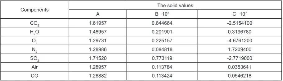
(11)

where: A, B, C – constant values, t – temperature, ºC.

The solid values to calculations of average proper warmth for individual components of gas and air and the fumes summarized in Table 1.

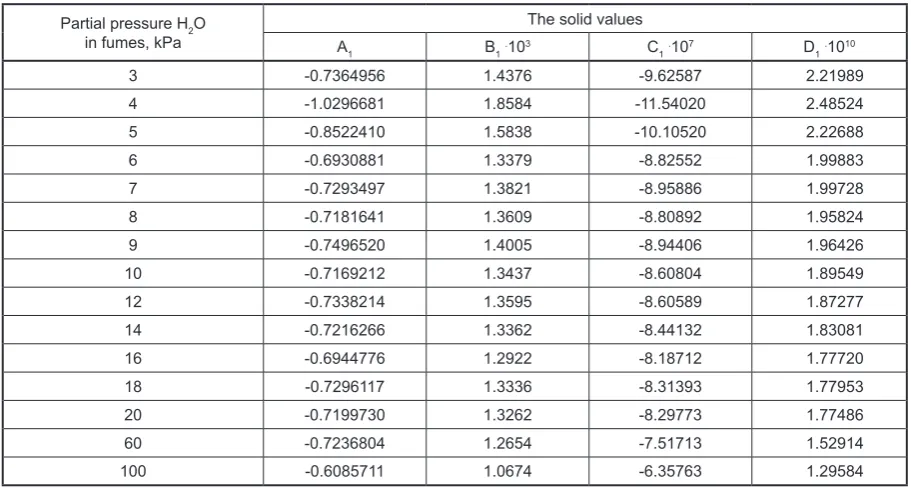
The dissociation coefficients represent a function of temperature and partial pressure being depend -ent on the CO₂ and H₂O contents of combustion gas. The energy balance equation enabling computa-tions to be performed with the method presented herein and the problems related to the dissociation of CO₂ and H₂O are described in a greater detail in references [7–9]. For particular partial pressure ranges, relationships for the dissociation coefficients as a function of temperature were developed. The general relationship adopts the following form:

3 1 2 1 1

1

B

t

C

t

D

t

A

+

⋅

+

⋅

+

⋅

=

a

(12)

where: A₁, B₁, C₁, D₁ – constant values.

The solid values to calculations of dissociation H₂O coefficients for individual ranges of partial pres -sure summarized in Table 2.

Components The solid values

A B . ₁₀3 _C . ₁₀7

CO2 1.61957 0.844664 -2.5154100

H2O 1.48957 0.201901 0.3196780

O2 1.29731 0.225157 -4.6761200

N2 1.28986 0.084818 1.7209400

SO2 1.71520 0.773119 -2.7719800

Air 1.28957 0.113784 0.0353641

CO 1.28882 0.113424 0.0546218

63

Advances in Science and Technology – Research Journal vol. 7 (18) 2013

The solid values to calculations of dissociation H₂O coefficients for individual ranges of partial pres -sure summarized in Table 3.

Using the described mathematical functions allowing for the effect of temperature, the dissociation

coefficients were determined from the relationships: sp

r

kal

i

_c

i

t

=

0

+

₍₁₎

" s

d

V

Q

i

₀

=

(2)

(

₉

)

₁₀

3

2500

10400

8

144030

33900

_

⋅











₊

_⋅

₋

₋











 −

⋅

+

⋅

=

c

h

o

s

w

h

Q

d c

(3)

" min s paliwa paliwa p pow a r

_V

t

c

t

c

V

i

=

⋅

⋅

+

⋅

(4)

sp d r

teor

i

_c

i

i

t

=

α

+

−

₍₅₎

" s d

V

Q

i

_α

=

(6)

O H O H CO CO

d r r

i =12470⋅

α

₂ ⋅ ₂ +10620⋅

α

₂ ⋅ ₂

(7)

O H

CO ,r

r _{2 2}

O H CO2,

α

2

α

teor

rzecz

t

t

=

µ

⋅

(8)

c

paliwa c h o n s p w

c =0.708⋅ +14.195⋅ +0.915⋅ +1.039⋅ +0.699⋅ +0.795⋅ +4.186⋅

∑

⋅ = ci r_i

c

(10)

2

t

C

t

B

A

c

i

=

+

⋅

+

⋅

(11)

3 1 2 1 1

1

B

t

C

t

D

t

A

+

⋅

+

⋅

+

⋅

=

α

( ) 2

{

(

2 ( ) 2

)

[

( ) 2 2

]

}

2 i 1 CO iCO i 1 CO i 1CO CO

CO

=

α

+

+

α

−

α

+

⋅

p

+

−

p

α

( )i HO

{

(

iHO ( )i HO

)

[

( )i HO HO

]

}

O

H2

=

α

+1 2

+

α

2

−

α

+1 2

⋅

p

+1 2

−

p

2

α

2

CO i

α

,

α

iH2O

( )i+1 CO2

α

,

α

( )i+1 H2O

2

CO

p

,

pH2O

( )i 1CO2

p +

,

p( )i+1H2O

(13)

sp r

kal

i

_c

i

t

=

0

+

₍₁₎

" s d

V

Q

i

₀

=

(2)

(

₉

)

₁₀

3

2500

10400

8

144030

33900

_

⋅











−

−

⋅

+











 −

⋅

+

⋅

=

c

h

o

s

w

h

Q

d c

(3)

" min s paliwa paliwa p pow a r

V

t

c

t

c

V

i

=

⋅

⋅

+

⋅

(4)

sp d r

teor

i

_c

i

i

t

=

α

+

−

₍₅₎

" s

d

V

Q

i

_α

=

(6)

O H O H CO CO

d r r

i =12470⋅

α

₂ ⋅ ₂ +10620⋅

α

₂ ⋅ ₂

(7)

O H CO ,r

r _{2 2}

O H CO2,

α

2

α

teor

rzecz

t

t

=

µ

⋅

(8)

c

paliwa c h o n s p w

c =0.708⋅ +14.195⋅ +0.915⋅ +1.039⋅ +0.699⋅ +0.795⋅ +4.186⋅

∑

⋅

= ci r_i

c

(10)

2

t

C

t

B

A

c

i

=

+

⋅

+

⋅

(11)

3 1 2 1 1

1

B

t

C

t

D

t

A

+

⋅

+

⋅

+

⋅

=

α

( ) 2

{

(

2 ( ) 2

)

[

( ) 2 2

]

}

2 i 1 CO iCO i 1 CO i 1CO CO

CO

=

α

+

+

α

−

α

+

⋅

p

+

−

p

α

( )i HO

{

(

iHO ( )i HO

)

[

( )i HO HO

]

}

O

H2

=

α

+1 2

+

α

2

−

α

+1 2

⋅

p

+1 2

−

p

2

α

2

CO i

α

,

α

iH2O

( )i+1CO2

α

,

α

( )i+1 H2O

2

CO

p

,

pH2O

( )i 1CO2

p +

,

p( )i+1H2O

(14) where:

sp r

kal

i

_c

i

t

=

0

+

₍₁₎

" s d

V

Q

i

₀

=

(2)

(

₉

)

₁₀

3

2500

10400

8

144030

33900

_

⋅











−

−

⋅

+











 −

⋅

+

⋅

=

c

h

o

s

w

h

Q

d c

(3)

" min s paliwa paliwa p pow a r

_V

t

c

t

c

V

i

=

⋅

⋅

+

⋅

(4)

sp d r

teor

i

_c

i

i

t

=

α

+

−

₍₅₎

" s

d

V

Q

i

_α

=

(6)

O H O H CO CO

d r r

i =12470⋅

α

₂ ⋅ ₂ +10620⋅

α

₂ ⋅ ₂

(7)

O H CO ,r

r _{2 2}

O H CO2,

α

2

α

teor

rzecz

t

t

=

µ

⋅

(8)

c

paliwa c h o n s p w

c =0.708⋅ +14.195⋅ +0.915⋅ +1.039⋅ +0.699⋅ +0.795⋅ +4.186⋅

∑

⋅

= ci r_i

c

(10)

2

t

C

t

B

A

ci

=

+

⋅

+

⋅

(11)

3 1 2 1 1

1

B

t

C

t

D

t

A

+

⋅

+

⋅

+

⋅

=

α

( ) 2

{

(

2 ( ) 2

)

[

( ) 2 2

]

}

2 i 1 CO iCO i 1 CO i 1CO CO

CO

=

α

+

+

α

−

α

+

⋅

p

+

−

p

α

( )i HO

{

(

iHO ( )i HO

)

[

( )i HO HO

]

}

O

H2

=

α

+1 2

+

α

2

−

α

+1 2

⋅

p

+1 2

−

p

2

α

2

CO i

α

,

α

iH2O

( )i+1CO2

α

,

α

( )i+1 H2O

2

CO

p

,

pH2O

( )i 1CO2

p +

,

p( )i+1H2O

– the coefficients of dissociation of CO₂ and H₂O for the lower partial pres- sure value from the range under consideration,

Table 2. The solid empirical values to calculations of dissociation CO₂ coefficients for individual ranges of partial

pressure

Table 3. The solid values to calculations of dissociation H2O coefficients for individual ranges of partial pressure

Partial pressure CO2 in fumes, kPa

The solid values

A1 B1.103 C1.107 D1.1010

3 1.0769795 -1.5647 5.62075 0

4 1.2074031 -1.6814 5.83561 0

5 1.2856280 -1.7473 5.93966 0

6 1.3233584 -1.7727 5.94880 0

7 1.3760369 -1.8167 6.01631 0

8 1.3985608 -1.8310 6.01588 0

9 1.4233874 -1.8483 6.02667 0

10 1.4440101 -1.8628 6.03492 0

12 1.4567568 -1.8623 5.98104 0

14 1.4782624 -1.8732 5.96471 0

16 1.4724573 -1.8583 5.89191 0

18 1.4510133 -1.8272 5.78002 0

20 1.4630247 -1.8325 5.76571 0

60 -0.0158115 0.4452 -5.45004 1.72170

100 -0.1273187 0.5825 -5.83210 1.69451

Partial pressure H2O in fumes, kPa

The solid values

A1 B1.103 C1.107 D1.1010

3 -0.7364956 1.4376 -9.62587 2.21989

4 -1.0296681 1.8584 -11.54020 2.48524

5 -0.8522410 1.5838 -10.10520 2.22688

6 -0.6930881 1.3379 -8.82552 1.99883

7 -0.7293497 1.3821 -8.95886 1.99728

8 -0.7181641 1.3609 -8.80892 1.95824

9 -0.7496520 1.4005 -8.94406 1.96426

10 -0.7169212 1.3437 -8.60804 1.89549

12 -0.7338214 1.3595 -8.60589 1.87277

14 -0.7216266 1.3362 -8.44132 1.83081

16 -0.6944776 1.2922 -8.18712 1.77720

18 -0.7296117 1.3336 -8.31393 1.77953

20 -0.7199730 1.3262 -8.29773 1.77486

60 -0.7236804 1.2654 -7.51713 1.52914

Advances in Science and Technology – Research Journal vol. 7 (18) 2013

64

1 sp kal

_c

" s d

V

Q

i

₀

=

(2)

(

₉

)

₁₀

3

2500

10400

8

144030

33900

_

⋅











−

−

⋅

+











 −

⋅

+

⋅

=

c

h

o

s

w

h

Q

d c

(3)

" min s paliwa paliwa p pow a r

_V

t

c

t

c

V

i

=

⋅

⋅

+

⋅

(4)

sp d r

teor

i

_c

i

i

t

=

α

+

−

₍₅₎

" s

d

V

Q

i

_α

=

(6)

O H O H CO CO

d r r

i =12470⋅

α

₂ ⋅ ₂ +10620⋅

α

₂ ⋅ ₂

(7)

O H CO ,r

r _{2 2}

O H CO2,

α

2

α

teor

rzecz

t

t

=

µ

⋅

(8)

c

paliwa c h o n s p w

c =0.708⋅ +14.195⋅ +0.915⋅ +1.039⋅ +0.699⋅ +0.795⋅ +4.186⋅

∑

⋅

= ci r_i

c

(10)

2

t

C

t

B

A

ci

=

+

⋅

+

⋅

(11)

3 1 2 1 1

1

B

t

C

t

D

t

A

+

⋅

+

⋅

+

⋅

=

α

( ) 2

{

(

2 ( ) 2

)

[

( ) 2 2

]

}

2 i 1 CO iCO i 1 CO i 1CO CO

CO

=

α

+

+

α

−

α

+

⋅

p

+

−

p

α

( )i HO

{

(

iHO ( )i HO

)

[

( )i HO HO

]

}

O

H2

=

α

+1 2

+

α

2

−

α

+1 2

⋅

p

+1 2

−

p

2

α

2

CO i

α

,

α

iH2O

( )i+1CO2

α

,

α

( )i+1 H2O

2

CO

p

,

pH2O

( )i 1CO2

p +

,

p( )i+1H2O

– the coefficients of dissociation of CO₂ and H₂O for the higher partial pressure value from the range under consideration,

1

sp r

kal

_c

t

=

0

₍₁₎

" s d

V

Q

i

₀

=

(2)

(

₉

)

₁₀

3

2500

10400

8

144030

33900

_

⋅











−

−

⋅

+











 −

⋅

+

⋅

=

c

h

o

s

w

h

Q

d c

(3)

" min s paliwa paliwa p pow a r

_V

t

c

t

c

V

i

=

⋅

⋅

+

⋅

(4)

sp d r

teor

i

_c

i

i

t

=

α

+

−

₍₅₎

" s

d

V

Q

i

_α

=

(6)

O H O H CO CO

d r r

i =12470⋅

α

₂ ⋅ ₂ +10620⋅

α

₂ ⋅ ₂

(7)

O H CO ,r

r _{2 2}

O H CO2,

α

2

α

teor

rzecz

t

t

=

µ

⋅

(8)

c

paliwa c h o n s p w

c =0.708⋅ +14.195⋅ +0.915⋅ +1.039⋅ +0.699⋅ +0.795⋅ +4.186⋅

∑

⋅ = ci r_i

c

(10)

2

t

C

t

B

A

ci

=

+

⋅

+

⋅

(11)

3 1 2 1 1

1

B

t

C

t

D

t

A

+

⋅

+

⋅

+

⋅

=

α

( ) 2

{

(

2 ( ) 2

)

[

( ) 2 2

]

}

2 i 1 CO iCO i 1 CO i 1CO CO

CO

=

α

+

+

α

−

α

+

⋅

p

+

−

p

α

( )i HO

{

(

iHO ( )i HO

)

[

( )i HO HO

]

}

O

H2

=

α

+1 2

+

α

2

−

α

+1 2

⋅

p

+1 2

−

p

2

α

2

CO i

α

,

α

iH2O

( )i+1CO2

α

,

α

( )i+1 H2O

2

CO

p

,

pH2O

( )i 1CO2

p +

,

p( )i+1H2O

– the actual partial pressure of CO₂ i H₂O, kPa,

1

sp

kal

_c

t

=

(1)

" s d

V

Q

i

₀

=

(2)

(

₉

)

₁₀

3

2500

10400

8

144030

33900

_

⋅











₊

_⋅

₋

₋











 −

⋅

+

⋅

=

c

h

o

s

w

h

Q

d c

(3)

" min s paliwa paliwa p pow a r

_V

t

c

t

c

V

i

=

⋅

⋅

+

⋅

(4)

sp d r

teor

i

_c

i

i

t

=

α

+

−

₍₅₎

" s

d

V

Q

i

_α

=

(6)

O H O H CO CO

d r r

i =12470⋅

α

₂ ⋅ ₂ +10620⋅

α

₂ ⋅ ₂

(7)

O H CO ,r

r _{2 2}

O H CO2,

α

2

α

teor

rzecz

t

t

=

µ

⋅

(8)

c

paliwa c h o n s p w

c =0.708⋅ +14.195⋅ +0.915⋅ +1.039⋅ +0.699⋅ +0.795⋅ +4.186⋅

∑

⋅ = ci r_i

c

(10)

2

t

C

t

B

A

c

i

=

+

⋅

+

⋅

(11)

3 1 2 1 1

1

B

t

C

t

D

t

A

+

⋅

+

⋅

+

⋅

=

α

( ) 2

{

(

2 ( ) 2

)

[

( ) 2 2

]

}

2 i 1 CO iCO i 1 CO i 1CO CO

CO

=

α

+

+

α

−

α

+

⋅

p

+

−

p

α

( )i HO

{

(

iHO ( )i HO

)

[

( )i HO HO

]

}

O

H2

=

α

+1 2

+

α

2

−

α

+1 2

⋅

p

+1 2

−

p

2

α

2

CO i

α

,

α

iH2O

( )i+1CO2

α

,

α

( )i+1 H2O

2

CO

p

,

pH2O

( )i 1CO2

p +

,

p( )i+1H2O – the higher CO₂ and H₂O partial pressure value from the range under con-

sideration, kPa.

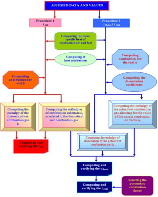
COMPUTATIONAL SOFTWARE PROGRAM

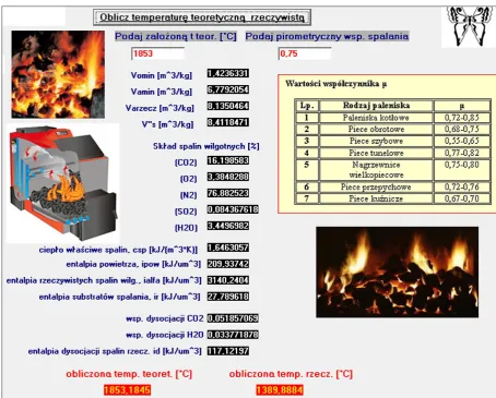
For developing the software program, computational procedures were employed, as illustrated in Figure 1. Considering the analytical relationships and the determined mathematical functions, a

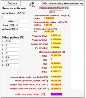
compu-tational software program has been developed, whose screenshot is shown in Figure 2.

According to the procedures shown in Figure 1, the input data in a form of the oxygen content of

combustion air, the excess air factor value, the temperatures of combustion air and fuel as well as fuel

composition needs to be entered in the program (Figure 3). The procedure for the calorimetric

tem-perature provides combustion process computation results for α = 1.0 and specific heats and enthalpies necessary for determining the temperature sought for (Figure 3). The assumed calorimetric temperature should be selected so that its value be approximate to the obtained result.

The procedure for the theoretical temperature provides combustion process computation results for the actual value of the excess air factor α and specific heats and enthalpies necessary for determining

Advances in Science and Technology – Research Journal vol. 7 (18) 2013

Fig. 2. A screenshot of program for calculations of combustion temperature of the solid fuels

Fig. 3. Part of the program window for input and calorimeter temperature

66

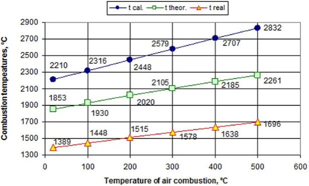
EXAMPLE COMPUTATION RESULTS

For the fuel composition shown in the pro

-gram window (Figure 3), the theoretical tempera-ture was computed for the variable value of the excess combustion air factor and the calorimetric, theoretical and actual temperatures for the vari-able combustion air temperature, with an excess combustion air factor of α = 1.2.

The computation results are summarized in

Figures 5 and 6. By examining Figure 5 it can be stated that with the increase in the excess air fac-tor value, the theoretical combustion temperature decreases, whereas increasing the air temperature

(Figure 6) causes an increase in the calorimetric,

theoretical and actual combustion temperatures.

SUMMARY

The paper has presented basic assumptions used for the development of a software program that will enable the user to determine the solid

Fig. 4. Part of the program window for theoretical and real temperature

fuel combustion temperature in an easy and expe-ditious manner. An asset of the program is the fact that, in addition to the ease of operation, provides the capability to readily change the input data in the form of the excess air factor value, combus-tion substrate temperature, fuel composicombus-tion and the oxygen fraction of the feed air. The possibility of entering a variable oxygen fraction is extreme-ly important in case of computation concerning combustion in an oxygen-enriched atmosphere.

For the actual temperature, it is also possible to select an appropriate pyrometric coefficient.

The presented computation results enable the authors to state that the theoretical and the actual combustion temperatures depend on the value of the excess air factor. With the increase in α, the

Advances in Science and Technology – Research Journal vol. 7 (18) 2013

The presented computational program can provide a useful tool for both teaching and re-search purposes. Indeed, combustion temperature computation results are an essential input data el-ement in the modelling of combustion processes, as well as in designing combustion chambers.

REFERENCES

1. Szargut J.: Termodynamika techniczna.

Wydawnic-two Politechniki Śląskiej, Gliwice 2010.

2. Pastucha L., Mielczarek E.: Podstawy termody-namiki technicznej. Wydawnictwo Politechniki

Częstochowskiej, Częstochowa 1998.

3. Kieloch M., Kruszyński S., Boryca J., Piechowicz Ł.: Termodynamika i technika cieplna – ćwiczenia

Fig. 5. The results of calculation of the theoretical combustion temperature

Fig. 6. The results of calculation of the calorimetric, theoretical and real combustion temperatures for variable of air temperature

rachunkowe, Skrypt. Wydawnictwo Politechniki

Częstochowskiej, Częstochowa 2006.

4. Senkara T.: Obliczenia cieplne pieców grzewczych w

hutnictwie. Wydawnictwo „Śląsk”, Katowice 1991.

5. Słupek S., Nocoń J., Buczek A.: Technika cieplna – ćwiczenia obliczeniowe. Wydawnictwo AGH,

Kraków 2002.

6. Nocuń J., Poznański J., Słupek S., Rywotycki M.: Technika cieplna, przykłady z techniki procesów

spalania, Uczelniane Wydawnictwo Naukowo- Dydaktyczne, Kraków 2007.

7. Szkarowski A.: Spalanie gazów, Wydawnictwo

Uc-zelniane Politechniki Koszalińskiej, Koszalin 2009.

8. Pudlik W.: Termodynamika. Wydawnictwo

Po-litechniki Gdańskiej, Gdańsk 2011.

9. Wiśniewski S.: Termodynamika techniczna, WNT,