www.geosci-model-dev.net/9/2549/2016/ doi:10.5194/gmd-9-2549-2016
© Author(s) 2016. CC Attribution 3.0 License.
Comparison of adjoint and nudging methods to initialise ice sheet
model basal conditions
Cyrille Mosbeux1,2, Fabien Gillet-Chaulet1,2, and Olivier Gagliardini1,2 1CNRS, LGGE, 38041 Grenoble, France
2Univ. Grenoble Alpes, LGGE, 38401 Grenoble, France
Correspondence to:Cyrille Mosbeux ([email protected]) Received: 12 January 2016 – Published in Geosci. Model Dev. Discuss.: 28 January 2016 Revised: 20 May 2016 – Accepted: 6 June 2016 – Published: 27 July 2016
Abstract.Ice flow models are now routinely used to forecast the ice sheets’ contribution to 21st century sea-level rise. For such short term simulations, the model response is greatly af-fected by the initial conditions. Data assimilation algorithms have been developed to invert for the friction of the ice on its bedrock using observed surface velocities. A drawback of these methods is that remaining uncertainties, especially in the bedrock elevation, lead to non-physical ice flux diver-gence anomalies resulting in undesirable transient effects. In this study, we compare two different assimilation algorithms based on adjoints and nudging to constrain both bedrock fric-tion and elevafric-tion. Using synthetic twin experiments with re-alistic observation errors, we show that the two algorithms lead to similar performances in reconstructing both variables and allow the flux divergence anomalies to be significantly reduced.
1 Introduction
Robustly reproducing the responsible mechanisms and fore-casting the ice sheets’ contribution to 21st century sea-level rise is one of the major challenges in ice sheet and ice flow modelling as highlighted by community-organised efforts such as SeaRISE (Sea-level Response to Ice Sheet Evolu-tion) (Bindschadler et al., 2013; Nowicki et al., 2013a, b) or ice2sea (e.g. Gillet-Chaulet et al., 2012; Shannon et al., 2013; Edwards et al., 2014).
Such projections on decadal timescales are sensitive to the model initial state which can account for an important source of uncertainty in the model response (Aðalgeirsdóttir et al., 2014). Improving the reliability of the model
projec-tions requires the model initial state to be better constrained from observations. The problem is that observations are of-ten uncertain, sparse in time and space, and indirect, so that the model state depends on many poorly determined physi-cal parameters and boundary conditions. Gradient-based op-timisation methods, such as the control method (MacAyeal, 1993) or the Robin inverse method (Arthern and Gudmunds-son, 2010), are efficient means to constrain such model pa-rameters and boundary conditions. These methods have been implemented and applied with success in ice flow models of different complexity in order to infer the basal drag, one of the most uncertain model parameters (e.g. Morlighem et al., 2010; Jay-Allemand et al., 2011; Schäfer et al., 2012; Gillet-Chaulet et al., 2012).
tens of metres to several hundreds of metres depending on the distance to observations and local topographic variability (Fretwell et al., 2013; Bamber et al., 2013). For comparison, the uncertainty on the surface elevation is usually 1 order of magnitude lower (Fretwell et al., 2013).
Because of theses large uncertainties, several methods have been proposed to consider the bedrock elevation as an optimisation variable. For example, Morlighem et al. (2011) derived the adjoint of the continuity equation for the ice thickness. The depth-averaged velocities and surface mass balance are then optimised to minimise the mismatch be-tween modelled and measured ice thicknesses. Surface ve-locity measurements are used as initial guess for depth-averaged velocities, and (by construction) the flux divergence produced by this approach is in equilibrium with the pre-scribed surface mass balance. However, there is no constraint that the optimised velocities are a solution of the stress equi-librium equations, so that, in general, the above method does not guarantee that the flow divergence anomalies resulting from an ice flow model initialised with the optimised fields will be reduced.
In their work, van Pelt et al. (2013) developed an itera-tive algorithm where the discrepancy between the surface el-evation predicted by the model and the observations is used to correct the bedrock elevation. Thus, the method does not rely on the accurate computation of the derivative of a cost function, as in a control method, and is then more similar to nudging methods that have been widely studied in the past decades in meteorology (e.g. Hoke and Anthes, 1976) and later in oceanography (Verron, 1992; Blayo et al., 1994). However, the method proposed by van Pelt et al. (2013) does not use observed surface velocities to control the model pa-rameters.
Several methods have been explored to construct model states where both the basal friction and the basal topogra-phy are treated as optimisation variables. In a pioneer work, Thorsteinsson et al. (2003) developed a least-squares inver-sion using analytical solutions for the transmisinver-sion of small-scale basal perturbations to the ice surface. This method has been extended in a non-linear Bayesian framework by Ray-mond and Gudmundsson (2009) and applied to an Antarc-tic ice stream by Pralong and Gudmundsson (2011). Bonan et al. (2014) have tested the performances of an ensemble Kalman filter on twin experiments using a shallow-ice flow-line model. The adjoint method has been tested by Goldberg and Heimbach (2013) and Perego et al. (2014) with models of different complexity. All these methods usually show good performance in reconstructing both basal friction and basal topography when using observations of both surface eleva-tion and surface velocities, so that mixing between the two variables does not seem to be too problematic for realistic ap-plications (Gudmundsson and Raymond, 2008). In addition, Pralong and Gudmundsson (2011) and Perego et al. (2014) show better performance when the rates of surface elevation change are also constrained from observations.
In this paper, we explore two different algorithms to in-fer both the basal friction and the basal topography and ini-tialise the model state using simultaneous observations at a given time. The first algorithm is in line with Goldberg and Heimbach (2013) and Perego et al. (2014) since it uses the adjoint solution of the force balance equation. We use the shallow shelf approximation to facilitate the derivation of the adjoint. Indeed, in this case the ice thickness appears as a state variable, while it changes the geometry of the do-main for higher order approximations (Perego et al., 2014). In its simplest formulation, the algorithm minimises the mis-fit between model and observed surface velocities, but an additional constraint where the flux divergence is close to a given surface mass balance can be added. The second method is an algorithm combining inversion of basal friction using the adjoint method and nudging of the bedrock topography. The control from the surface velocity observations is im-posed by the adjoint step while the nudging step allows to decrease the discrepancy between the flux divergence and the surface mass balance. The main motivation of this sec-ond algorithm is its ease of implementation as no inversion of the model with respect to the ice thickness is required. Our objective is then to illustrate its ability to reconstruct the bedrock topography by comparison with the results of the more mathematically founded first algorithm. Both al-gorithms are implemented in the finite element ice sheet/ice flow model Elmer/Ice (Gagliardini et al., 2013). The meth-ods and algorithms are described in details in Sect. 2. To test their performances, we design a twin experiment in Sect. 3. The results are discussed in Sect. 4.
2 Methods 2.1 Direct model
For the force balance, we use the standard vertically integrated shallow shelf approximation (SSA) equations (MacAyeal, 1989). This approximation neglects the effects of vertical shearing and is, hence, more adapted to model the flow in areas where the friction is low, resulting in an ice mo-tion dominated by sliding. The horizontal velocity field(u, v) is a solution of
∂
∂x
2H ν
2∂u ∂x+ ∂v ∂y + ∂ ∂y H ν ∂v ∂x+ ∂u ∂y
−βu=ρgH∂zs ∂x ∂ ∂x H ν ∂v ∂x+ ∂u ∂y + ∂ ∂y
2H ν
∂u ∂x+2
∂v ∂y
−βv=ρigH ∂zs
∂y, (1)
H=zs−zbthe thickness, withzsandzbthe top and bottom surface elevations, respectively.
Natural boundaries are the calving fronts where the Neu-mann condition results from the difference between the ice pressure and the sea water pressure:
4H ν∂u
∂xnx+2H ν ∂v
∂ynx+H ν( ∂u ∂x+
∂v ∂x)ny =(ρigH−ρwgH0)nx
4H ν∂v
∂yny+2H ν ∂v
∂xny+H ν( ∂u ∂x+
∂v ∂x)nx
=(ρigH−ρwgH0)ny, (2)
whereρwis the water density,H0the ice thickness below sea level, and nx andny the two components of the horizontal
unit vector normal to the calving front. Dirichlet boundary conditions are prescribed for other non-natural boundaries. The continuity equation for the ice thickness is given by
∂H ∂t +
∂(uH )
∂x +
∂(vH )
∂y =a, (3)
where a is the surface mass balance and accumula-tion/ablation at the bedrock interface is neglected.
2.2 Inverse methods
The objective of the methods is to produce a model state from Eq. (1) that best fits the observations of surface velocities and the rates of change of ice thickness. To minimise the discrep-ancy between the model and the observations, the optimisa-tion parameter vectorpcontains both the basal friction coef-ficientβand the bedrock elevationzb(p=(β, zb)). 2.2.1 Cost functions
The misfit between the model and the corresponding obser-vations is evaluated using cost functions. The first cost func-tion measures the difference between modelled (u) and ob-served (uobs) surface velocities:
Jv=
Z
0
1
2(|u−uobs|)
2d0, (4)
where0is the model domain.
The second cost function measures the misfit between modelled and observed thickness rates of change:
Jdiv=
Z 0 1 2 ∂H ∂t − ∂H ∂t obs 2
d0. (5)
The modelled rate of change of ice thickness ∂H /∂t is evaluated from Eq. (3) as the difference between the flux di-vergence solution of Eq. (1) and the prescribed surface mass balance. Observed rate of change of ice thickness(∂H /∂t )obs
can be estimated from surface elevation trends extracted from radar altimetry measurements (Flament and Rémy, 2012).
In general, both Eqs. (4) and (5) could be weighted with error covariance estimates such as the one of Flament and Rémy (2012). However, this information is not often avail-able. In this paper, observed ice surface velocities (uobs) and observed rate of change of ice thickness(∂H /∂t )obsare con-sidered perfectly known or perturbed with a Gaussian noise which would make unnecessary the addition of a covariance term.
The objective is then to find the parameter vectorpthat minimisesJvandJdiv. This can be achieved in different ways as illustrated in the following sections.
2.2.2 Adjoint method
The two cost functions have an implicit dependence on the parameter vectorp through the model surface velocitiesu which are solutions of Eq. (1). The gradient of the cost func-tions with respect topcan be computed efficiently using the adjoint equations of Eq. (1). The derivation of the continuous adjoint equations and the gradient ofJvwith respect to the friction coefficientβcan be found in MacAyeal (1993). This can be easily extended for the computation of the gradient with respect toH.
The implementation in Elmer/Ice is carried out in a way that stays as close as possible to the differentiation of the discrete implementation of the direct equations. This method should lead to a better accuracy on the gradient computation than the discretisation of the continuous equations. Elmer/Ice uses programming features that are not supported by auto-matic differentiation tools and the differentiation of the cru-cial parts of the discrete source code (e.g. cost function com-putation, matrix assembly) has been done manually. If the problem is non-linear, as here due to the dependence of the viscosity to the strain rate, and the non-linearity solved using a Picard iterative scheme, the iterations should be reversed (at least partially) in the adjoint code to achieve a good accuracy of the computed gradient (Martin and Monnier, 2013). How-ever, as the present direct solver is equipped with a Newton linearisation of the ice viscosity so that it remains self-adjoint (Petra et al., 2012), the Newton iterations are not reversed in the adjoint code and we only keep the last iteration. The ad-joint code has been validated on standard tests by compar-ing the gradients with those obtained from a finite difference evaluation. The agreement is usually better than 0.1 %.
Inverse problems are often ill-posed, leading to instabil-ities. It is then necessary to add regularisation terms to the cost function to avoid overfitting of data. This can be done in the form of a Tikhonov regularisation. Here, we define two different regularisations. The first one measures the norm of the first spatial derivative of the componentpi ofp, thus
Jregi= 1 2 Z 0 ∂p i ∂x 2 + ∂p i ∂y 2
d0. (6)
The second forces the optimisation variables to stay close to a certain prior or background informationpb. This back-ground can be based on observations or on empirical knowl-edge. This second regularisation term is written as
Jbi=
1 2 Z 0 1 σ2 p
(pi−pi,b)2d0, (7)
whereσpis a spatial parameter allowing to give more or less weight to the prior informationpi,b.
The computation of the gradients of these two functionals with respect to pis trivial. How these regularisation terms are weighted with respect to the model–data misfit function-als Eqs. (4) and (5) is described in more details with the de-scription of the algorithms in Sec. 2.3.
This minimisation is achieved using the quasi-Newton routine M1QN3 (Gilbert and Lemaréchal, 1989) imple-mented in Elmer/Ice. This method uses an approximation of the second derivatives of the cost function and is therefore more efficient than a fixed-step gradient descent.
2.2.3 Nudging method
By definition, the steady-state solution of Eq. (3) where a is replaced by the apparent mass balancea−(∂H /∂t )obsis the minimum for Jdiv. Running the model forward in time with a constant forcing is then a simple way to minimise Jdiv, equivalent to a relaxation step. Here, we assume that the surface elevation is known so that computed changes in ice thickness are used to correct the bedrock elevationzb. Dur-ing this process, the ice thickness can substantially deviate from observations. Nudging methods, also called Newtonian relaxation, can remedy to this problem by constraining the thickness to fit observations through an additional callback term in Eq. (3), which now writes
∂H ∂t +
∂(uH )
∂x +
∂(vH ) ∂y =a−
∂H
∂t
obs
−k(H−Hobs), (8)
where the coefficientkdefines the amplitude of the callback at each node of the model. These methods imply a trade-off, adjustable through k, between model physics and observa-tions. The callback term can depend on many different crite-ria such as observation accuracy or distance to observation (Hoke and Anthes, 1976). Here, we take k as a Gaussian function of the distance to the closest observation so that the callback is maximum where an observation is available and decreases to zero far from all observations. The choice of the variance for the Gaussian function is discussed in Sect. 4.2.
2.3 Algorithms
From the methods presented in the previous section we de-sign two algorithms to infer simultaneously the friction co-efficientβ and the bedrock elevationzb. To ensure that the friction coefficient remains positive during the inversion, we use the following change of variable
β=10α. (9)
2.3.1 Adjoint method with two parameters (ATP) This algorithm uses the gradients of the cost functions de-rived using the adjoint method to optimise bothαandzb. For the regularisation, a constraint on the smoothness is imposed forαusing Eq. (6) while a constraint on the background in-formation is imposed forzbusing Eq. (7). The total cost func-tion then writes
JATP(α, zb)=Jv+γ Jdiv+λαJregα+λzbJbzb, (10)
whereγis a constant fixed to give a similar weight toJvand Jdiv whileλα andλzb are two constants allowing to adjust the weight given to the regularisation terms. Following Fürst et al. (2015), several pairs (λα,λzb) are tested using a L-curve approach, and optimal values are taken from the combina-tions that avoid two extremes: overfitting of the observacombina-tions or excessive regularisation.
2.3.2 Adjoint-nudging coupling (ANC)
In this algorithm, the adjoint method is first used to optimise αonly by minimising the following total cost function JANC(α)=Jv+γ Jdiv+λαJregα. (11) The bedrock elevation is then updated using the nudging method by solving Eq. (8) for a given time period T. T should be neither too short nor too long to allow to reduce Jdiv without overfitting observations. The sensitivity of the method toT is discussed in the results section.
These two steps are then repeated iteratively until changes inJvandJdivbetween two iterations are less than 1 %.
3 Manufactured data sets
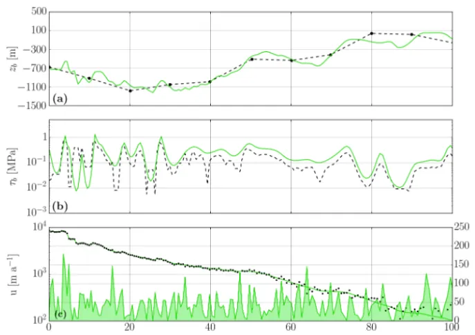
Figure 1.Reference (solid lines) and initial (dashed lines) state for(a)the bedrock elevationszb,(b)the estimated basal tractionτb=βu,
and(c)the surface velocities. In(a), synthetic observations every 10 km are the plain black circles. In(c)the observed velocities are depicted by the circles and the shaded green curve is the absolute difference between observed and reference surface velocities (right axis).
3.1 Reference experiment
A flowline of Jakobshavn Glacier, Greenland, is used to test the two algorithms with realistic conditions. Jakobshavn Is-brae is one of Greenland’s three largest outlet glaciers and has one of the largest drainage basin on the ice sheet’s west-ern margin (Bindschadler, 1984). It is also the fastest Green-land glacier with a terminus velocity greater than 13 km a−1 (Joughin et al., 2008, 2014). The flowline is 550 km long and runs from the ice divide to the ice front. The surface and bedrock elevations are taken from available digital elevation models (Bamber et al., 2013). The basal friction coefficient field is first adjusted so that the model velocities fit observed velocities (Joughin et al., 2010). To have realistic thickness rates of change, the free surface is relaxed to steady state. The surface mass balance a in Eq. (3) has been calibrated so that the steady state is close to the initial geometry, and is meant to take into account the flow convergence or diver-gence along the flowline. The steady-state solution is used as the reference of the twin experiment.
The geometry is discretised through a mesh of 500 linear elements, increasingly refined to the front of the glacier. The element size decreases from∼2 km in the upper part of the glacier to∼400 m down to the front.
Results will only be presented on the first 100 km upstream of the glacier front where velocities are above 100 m a−1and where the SSA is more appropriate but the inversion is done all along the flowline up to the ridge.
3.2 Synthetic observations
Synthetic observations are generated by sampling and/or adding noise to the reference simulation. Details for each required field are given below. These synthetic observations and initial fields for the inverse methods are compared to the reference in Fig. 1.
3.2.1 Surface velocities
Surface velocities are assumed to be observed at the same resolution as the reference simulation but with a white Gaus-sian noise with a meanµ=0 and a standard deviationσ= 50 m a−1. This corresponds to a root mean squared (rms) er-ror of 47.8 m a−1for the entire flowline. The reference and noisy observed surface velocities are shown in Fig. 1c to-gether with their absolute difference.
3.2.2 Surface mass balance and thickness rate of change
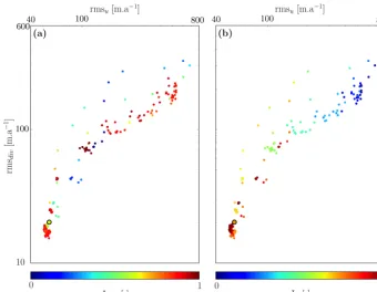
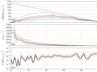
Figure 2. Mean error on the thickness rate of change (rmsdiv) as a function of the mean error on velocity (rmsu) for the 255 pairs of
regularisation parameters (λα,λzb). Colour scales show the normalised regularisation terms(a)Jregα and(b)Jzb (0 corresponds with the
lowest value and 1 with the highest value obtained with the 255 pairs). The chosen value (λα=1011,λzb=107) is shown with a black circle.
3.2.3 Surface and bedrock elevations
The surface elevation is assumed to be perfectly observed. For the bedrock elevationzb, we simulate observations rep-resenting airborne radar measurements crossing the flowline. Bedrock elevations are sampled every 10 km with a Gaus-sian noise centred on zero and with a standard deviation of σ =50 m. This leads to a rms error of 62.4 m on the 55 ob-servation points of the entire flowline. This error is similar to the errors given in practice on recent bedrock elevation maps (Fretwell et al., 2013; Bamber et al., 2013). For the mesh nodes between the observations, the bedrock is linearly in-terpolated as shown in Fig. 1a. This is used as the first guess for the inverse methods and as the background information for the regularisation in Eq. (7).
3.2.4 Model parameters
The ice viscosity is assumed to be perfectly known and cor-responds to the viscosity used in the reference experiment.
Assuming that no observation of the friction coefficient is available, an initial solution has to be postulated. A good first guess forβis provided by using the driving stress to estimate the basal shear stress:
βini(x)=
ρigH (x)|θ (x)|
|u(x)| , (12)
whereH (x),θ (x), andu(x)are, respectively, the ice thick-ness, the surface slope and the surface velocity at positionx. The reference and initial values are shown in Fig. 1b.
The rms errors on the surface velocities and the rate of change of ice thickness between the initial state and the syn-thetic observations are, respectively, 761 and 357 m a−1.
The average relative error on the basal shear stress is mea-sured as
ετb = 1 L
Z
0
|τb| − |τb,ref| |τb,ref|
d0, (13)
whereτb,ref is the basal shear stress in the reference experi-ment andLthe length of the flowline. The relative error on the basal shear stress with our initial estimate of the basal friction βini is 394 %. The performances of the two algo-rithms in reducing these initial errors are presented in the following section and will be compared to these initial er-rors.
4 Results
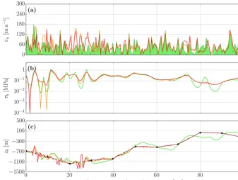
Figure 3.Results of the ATP algorithm with (orange) and without (red) optimisation ofJdiv, i.e.γ=1 orγ=0, respectively, in Eq. (10): (a)absolute difference between observed and model velocities,(b)estimated basal traction, and(c)estimated bedrock elevation. The green shaded area is the difference between the noisy reference velocities and the true velocities. The green solid lines are the reference values and the black dashed line is the initial guess for the bedrock elevation.
λzb) is given in Fig. 2. Both graphs show that most of the pairs fitting well the observed velocities can also adequately reproduce the observed rate of change of the ice thickness. Figure 2b also shows that smaller misfits onJzb clearly in-volve higher rms misfits on the ice surface velocities (rmsu)
and on the rate of change of the ice thickness (rmsdiv). On the contrary, Fig. 2a does not show a clear relation between the magnitude ofJregαand the magnitude of rmsuand rmsdiv.
Both graphs also show a high density of pairs for small rmsu
and rmsdiv. However, the pair (λα=1011,λzb =10
7) seems to come off the others, giving a good trade off between data fitting and regularisation. Notice that the constantγ is fixed to 1 sinceJvandJdivhave the same order of magnitude.
The optimisation of bothαandzbsimultaneously allows a rms misfit of 49.7 m a−1on velocities to be reached, very similar to the observation rms error, showing no overfitting of velocity data. The rate of change of ice thickness misfit is also largely decreased with a rms value of 19.2 m a−1. The resulting basal traction τb andzb as well as the misfit for the surface velocities are given in Fig. 3. The basal traction variability is accurately reproduced with a corresponding av-erage relative misfit of only 25 % along the entire flowline with respect to the reference basal shear stressτb,ref, i.e. more than a 10-fold decrease of the initial misfit. We only notice local overestimations of slipperiness in bedrock pits without significant impacts on the flow velocities. Indeed, under a de-fined value ofβ corresponding to a nearly perfectly sliding
case, an additional reduction in friction has no impact on the flow. The same reasoning applies to a nearly perfectly sticky case, where an increased friction would not involve more de-crease of the velocity. The bedrock elevationzbis well recon-structed in the first 50 km upstream of the glacier front. The discrepancy with respect to the reference bedrock is larger upstream where the cost functionJvis less sensitive because of lower velocities. This could possibly be improved by us-ing a cost function measurus-ing the logarithm of the misfit as in Morlighem et al. (2010), but with a greater risk of fitting noise since the relative observation error is higher in these regions.
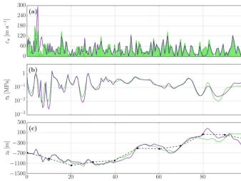
Figure 4.Results of the ANC algorithm (purple):(a)absolute difference between observed and model velocities,(b)estimated basal traction, and(c)estimated bedrock elevation. The green shaded area is the difference between the noisy reference velocities and the true velocities. The green solid lines are the reference values and the black dashed line is the initial guess for the bedrock elevation.
Introduction of a Gaussian noise on(∂H /∂t )obshas been investigated in order to assess its effect on the optimisation of Jdiv. Different levels of standard deviation σ have been tested. Results show that the optimisation is little affected by this noise even for standard deviationsσ going up to the same order of magnitude as the surface accumulationa. In-troduction of systematic bias on(∂H /∂t )obsin a physically acceptable range, i.e. of the same order of magnitude as sur-face accumulationa, also have few consequences on the op-timisation.
4.2 Adjoint-nudging coupling (ANC)
The steps for the optimisation ofαonly are conducted with a valueλα=5×10⁹, which allows a good agreement between
the different cost functions and a valueγ=1.
In addition to the regularisation parameters of Eq. (11), ANC algorithm depends on the time period for the nudg-ing steps T and the variance of the Gaussiank in Eq. (8). The nudging period T impacts the convergence on Jv and Jdiv after each cycle. The convergence is substantially simi-lar for T from 1 to 4 years. Longer periods mainly involve a worse minimisation ofJvsince there is no control on ve-locities during nudging. Shorter relaxation times do not in-volve sufficient change ofzbinducing a lower minimisation ofJdivfor a given number of cycles. Therefore, a relaxation timeT =1 year is adopted, which seems sufficient to allow significant changes ofzbwithout too much adaptation to the
previous intermediate value of the friction coefficient. The al-gorithm is stopped after 10 cycles, corresponding to the stop-ping criterion of Sect. 2.3.2. For a givenT period, tests show that variance values of the Gaussiankin Eq. (8) larger than 1 km are excessive and induce non-physical callback ampli-tudes when departing from observations. After a few cycles, the resulting bedrock induces an increase between modelled and observed velocities that cannot be overcome by the basal drag inversion. Variance smaller than 1 km has little impact on the final result in terms of cost functions. However, among the acceptable values, the 1 km variance gives the best agree-ment between misfit on the surface velocities and misfit on the rate of change of the ice thickness.
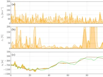
Figure 5.The five new references build from a 5-year perturbation of the initial reference by an increase of the friction parameter:β=2βref
(green),β=3βref(red),β=4βref(blue lines),β=5βref(purple), andβ=10βref(orange). New references for(a)the thickness rate of
change for the different perturbations,(b)velocities (without observation noise), and(c)friction coefficientsβ.
80 to 100 km to the front, strongly linked to the poorer fit of β (see Fig. 4).
As for ATP, introduction of a Gaussian noise in the ob-served thickness rate of change (∂H /∂t )obs has also been tested. Results show no significant impacts on the opti-misation. Nevertheless, introduction of systematic bias in (∂H /∂t )obs has direct consequences on the nudging steps inducing an offset of zb of the range of the systematic bias cumulated on the nudging periodT. ANC is therefore more sensitive to systematic bias than ATP.
4.3 Further sensitivity experiments
In order to evaluate the efficiency of both algorithms in transient states, we construct new reference cases where (∂H /∂t )obs6=0. This is achieved by multiplyingβref by a factor of 2, 3, 4, 5, and 10. As a consequence, increasing the basal friction involves a disequilibrium of the glacier, an ice thickening, and a decrease of ice flow velocities.
The time period for the glacier to come back to equi-librium, after this change of friction parameter, depends on the amplitude of the perturbation. Here, the perturbation is only applied during 5 years in order to keep the five cases in disequilibrium. Resulting thickness rates of change (∂H /∂t )obs6=0 are in the same order of magnitude as the tuned surface mass balancea. The five new reference cases are presented in Fig. 5.
Figure 6.Range of values for ATP algorithm for the five perturbations of the friction coefficientβ.(a, b)Minimum (dark orange shade) and maximum (light orange shade) of absolute difference between observed and model velocities and relative error forτb, respectively.(c)Range
of values for bedrock elevationzb(orange shade). The green solid line is the reference value and the black dashed line is the initial guess for
the bedrock elevation.
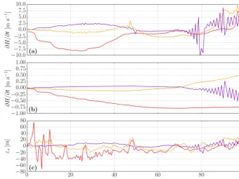
Figure 8.Evolution of∂H /∂tafter 1 year(a)and 10 years(b)of prognostic simulation and the resulting mismatch after 10 years between surfaces obtained with three different initial states and reference surface(c). The orange and purple lines give the results for ATP and ANC. The red line gives the result for inversion ofβonly.
4.4 Flow divergence in transient model
In this section, we assess the impact of our initialisation al-gorithms on the prognostic response of the model forward in time assuming the same constant forcing used to build the reference state. By doing so, if the initialisation was per-fect, one would expect no change of the geometry and ice flow during this prognostic simulation. The experiment is performed from ATP and ANC initial states. A third initial-isation state is constructed for which only the friction coef-ficient has been optimised, keepingzbequals to the a priori zbb. This third initialisation, called “β only” involves a rms misfit on velocities of 43.3 m a−1and an average relative er-rorετb,refof 36 % on basal shear stress, similar to the ATP and ANC initial states. However, the rms misfit on the thickness rate of change is significantly higher, 147.8 m a−1.
The prognostic simulations are conducted during a 10-year period in order to see how the initial thickness rate evolves during this time and how it impacts the final ice thickness and ice surface. The thickness rates of change after 1 and 10 years of simulation are shown in Fig. 8a and b, respectively, while the mismatch on the surface elevation after 10 years is shown in Fig. 8c.
ANC and ATP initial states involve thickness rates of change much closer to zero than the optimisation of “βonly”. This also leads to a lower mismatchεson the surface eleva-tion with respect to the reference after 10 years of simula-tion. Indeed, this mismatch is well below 20 m for both ANC
Figure 9.Ice surface elevationzsafter 10 years of prognostic
sim-ulation for three different initial states: initialisation with ATP algo-rithm (orange line), with ANC algoalgo-rithm (purple line), and with the inversion ofβonly (red line). The green line is the reference surface elevation. The figure focuses on the first 50 km next to the front of the glacier.
and ATP, except on a few kilometres in the upstream region, whereas the optimisation ofβ only gives rise to a mismatch globally above 20 m with some regions exceeding 50 m.
of low-scale variations of the surface elevation due to the transfer of similar variations from the bedrock elevation zb (Fig. 9). These variations tend to disappear with the optimi-sation of the friction only, giving rise to a lower resolution of the surface. However, we should point out that this direct transfer of bedrock variations to the surface is a consequence of the SSA ice flow model used and that a full Stokes model would produce a more diffusive transfer response.
5 Conclusions
The presented algorithms allow the reconstruction of two poorly known parameters: the bedrock topographyzband the friction coefficientβat the same time.
The optimisation of these two parameters mainly relies on the knowledge of some other data that are easier to measure: ice surface velocities and thickness rates of change. Some lo-cal measurements of bedrock elevation and associated errors are necessary in order to define a backgroundzb. The two al-gorithms aim to infer the set of parameters which minimises the misfit between the model and the corresponding observa-tions of ice surface velocities and thickness rates of change. If the optimisation of ice surface velocities is usually sufficient to inferβ, the inference of a second parameter requires more information to distinguish the effects of each parameters on the flow. Observations of rates of change of ice thickness are necessary to allow optimisingzbas well.
The two algorithms are based on the optimisation of the friction coefficientβ with the adjoint method. The bedrock geometry zb is reconstructed in two different ways, again with the adjoint method for the first algorithm (ATP) and with a nudging method based on mass conservation equation for the second one (ANC).
We have shown that the ATP algorithm is capable to well reproduceβ and the corresponding basal shear stresses, while the bedrock elevation zb is only well reproduced in high velocities regions. The lower the velocity, the harder for zbto depart from its initial background value. The iterative algorithm coupling adjoint method and nudging (ANC) gives results that are just as good. Moreover, ANC allows a better reconstruction of the bedrock geometry zbin most regions. This is a very good sign for an adaptation of the method to non-depth-integrated flow models such as full Stokes mod-els where the bedrock topography is no more a state variable but affects the domain geometry making the derivation of the adjoint even more demanding (Perego et al., 2014). Indeed, there is no need to inverse a shape variable like bedrock to-pography which is a usual obstacle to adjoint-based methods. Furthermore, the transient simulations over 10 years from initial states reconstructed with the two algorithms devel-oped give very encouraging results. The model divergence is clearly decreased with respect to usual inversion methods of the friction coefficient only. The integration of observa-tions like thickness rates variation through an optimisation
of the divergence during inversion or nudging steps, allows to regularise the solution in a physical way and also clearly improves the results.
Finally, the sensitivity experiments shows that the differ-ent algorithms can take into account the disequilibrium of mass balance, which is particularly interesting considering that a large amount of outlet glaciers in both Greenland and Antarctica present this feature.
6 Data availability
The construction of the twin experiment presented in this ar-ticle is partially based on real data. Surface velocities come from Joughin et al. (2010), while surface and bedrock ge-ometries come from Bamber et al. (2013). Notice that sur-face topography slightly differs from Bamber et al. (2013) in order to reach steady state. The simulations were performed using the Elmer/Ice finite element model (https://github.com/ ElmerCSC/elmerfem). Some modules were specially devel-oped for this application.
Acknowledgements. We would like to thank the editor, A. Le Brocq, as well as the two referees, S. L. Cornford and R. Arthern, for their positive and constructive comments which greatly improved the initial version of the manuscript. This work was supported by the French National Research Agency (ANR) un-der the SUMER (Blanc SIMI 6) 2012 project ANR-12-BS06-0018. LGGE is part of Labex OSUG@2020 (ANR10 LABX56).
Edited by: A. Le Brocq
Reviewed by: R. Arthern and S. L. Cornford
References
Aðalgeirsdóttir, G., Aschwanden, A., Khroulev, C., Boberg, F., Mottram, R., Lucas-Picher, P., and Christensen, J.: Role of model initialization for projections of 21st-century Greenland ice sheet mass loss, Biocontrol Sci. Techn., 60, 782–794, doi:10.3189/2014JoG13J202, 2014.
Arthern, R. J. and Gudmundsson, G. H.: Initialization of ice-sheet forecasts viewed as an inverse Robin problem, J. Glaciol., 56, 527–533, doi:10.3189/002214310792447699, 2010.
Bamber, J. L., Griggs, J. A., Hurkmans, R. T. W. L., Dowdeswell, J. A., Gogineni, S. P., Howat, I., Mouginot, J., Paden, J., Palmer, S., Rignot, E., and Steinhage, D.: A new bed elevation dataset for Greenland, The Cryosphere, 7, 499–510, doi:10.5194/tc-7-499-2013, 2013.
Bindschadler, R. A.: Jakobshavns Glacier drainage basin: A bal-ance assessment, J. Geophys. Res.-Oceans, 89, 2066–2072, doi:10.1029/JC089iC02p02066, 1984.
H., Seroussi, H., Takahashi, K., Walker, R., and Wang, W. L.: Ice-sheet model sensitivities to environmental forcing and their use in projecting future sea level (the SeaRISE project), J. Glaciol., 59, 195–224, doi:10.3189/2013JoG12J125, 2013.
Blayo, E., Verron, J., and Molines, J. M.: Assimilation of TOPEX/POSEIDON altimeter data into a circulation model of the North Atlantic, J. Geophys. Res., 99, 24691, doi:10.1029/94JC01644, 1994.
Bonan, B., Nodet, M., Ritz, C., and Peyaud, V.: An ETKF approach for initial state and parameter estimation in ice sheet modelling, Nonlin. Processes Geophys., 21, 569–582, doi:10.5194/npg-21-569-2014, 2014.
Durand, G., Gagliardini, O., Favier, L., Zwinger, T., and le Meur, E.: Impact of bedrock description on modeling ice sheet dynamics, Geophys. Res. Lett., 38, L20501, doi:10.1029/2011GL048892, 2011.
Edwards, T. L., Fettweis, X., Gagliardini, O., Gillet-Chaulet, F., Goelzer, H., Gregory, J. M., Hoffman, M., Huybrechts, P., Payne, A. J., Perego, M., Price, S., Quiquet, A., and Ritz, C.: Effect of uncertainty in surface mass balance–elevation feedback on pro-jections of the future sea level contribution of the Greenland ice sheet, The Cryosphere, 8, 195–208, doi:10.5194/tc-8-195-2014, 2014.
Flament, T. and Rémy, F.: Dynamic thinning of Antarctic glaciers from along-track repeat radar altimetry, J. Glaciol., 58, 830–840, doi:10.3189/2012JoG11J118, 2012.
Fretwell, P., Pritchard, H. D., Vaughan, D. G., Bamber, J. L., Bar-rand, N. E., Bell, R., Bianchi, C., Bingham, R. G., Blankenship, D. D., Casassa, G., Catania, G., Callens, D., Conway, H., Cook, A. J., Corr, H. F. J., Damaske, D., Damm, V., Ferraccioli, F., Fors-berg, R., Fujita, S., Gim, Y., Gogineni, P., Griggs, J. A., Hind-marsh, R. C. A., Holmlund, P., Holt, J. W., Jacobel, R. W., Jenk-ins, A., Jokat, W., Jordan, T., King, E. C., Kohler, J., Krabill, W., Riger-Kusk, M., Langley, K. A., Leitchenkov, G., Leuschen, C., Luyendyk, B. P., Matsuoka, K., Mouginot, J., Nitsche, F. O., Nogi, Y., Nost, O. A., Popov, S. V., Rignot, E., Rippin, D. M., Rivera, A., Roberts, J., Ross, N., Siegert, M. J., Smith, A. M., Steinhage, D., Studinger, M., Sun, B., Tinto, B. K., Welch, B. C., Wilson, D., Young, D. A., Xiangbin, C., and Zirizzotti, A.: Bedmap2: improved ice bed, surface and thickness datasets for Antarctica, The Cryosphere, 7, 375–393, doi:10.5194/tc-7-375-2013, 2013.
Fürst, J. J., Durand, G., Gillet-Chaulet, F., Merino, N., Tavard, L., Mouginot, J., Gourmelen, N., and Gagliardini, O.: Assim-ilation of Antarctic velocity observations provides evidence for uncharted pinning points, The Cryosphere, 9, 1427–1443, doi:10.5194/tc-9-1427-2015, 2015.
Gagliardini, O., Zwinger, T., Gillet-Chaulet, F., Durand, G., Favier, L., de Fleurian, B., Greve, R., Malinen, M., Martín, C., Råback, P., Ruokolainen, J., Sacchettini, M., Schäfer, M., Seddik, H., and Thies, J.: Capabilities and performance of Elmer/Ice, a new-generation ice sheet model, Geosci. Model Dev., 6, 1299–1318, doi:10.5194/gmd-6-1299-2013, 2013.
Gilbert, J. C. and Lemaréchal, C.: Some numerical experiments with variable-storage quasi-Newton algorithms, Math. Program., 45, 407–435, doi:10.1007/BF01589113, 1989.
Gillet-Chaulet, F., Gagliardini, O., Seddik, H., Nodet, M., Du-rand, G., Ritz, C., Zwinger, T., Greve, R., and Vaughan, D. G.: Greenland ice sheet contribution to sea-level rise from a
new-generation ice-sheet model, The Cryosphere, 6, 1561–1576, doi:10.5194/tc-6-1561-2012, 2012.
Goldberg, D. N. and Heimbach, P.: Parameter and state estima-tion with a time-dependent adjoint marine ice sheet model, The Cryosphere, 7, 1659–1678, doi:10.5194/tc-7-1659-2013, 2013. Gudmundsson, G. H. and Raymond, M.: On the limit to resolution
and information on basal properties obtainable from surface data on ice streams, The Cryosphere, 2, 167–178, doi:10.5194/tc-2-167-2008, 2008.
Hoke, J. E. and Anthes, R. A.: The Initialization of Nu-merical Models by a Dynamic-Initialization Technique, Mon. Weather Rev., 104, 1551–1556, doi:10.1175/1520-0493(1976)104<1551:TIONMB>2.0.CO;2, 1976.
Jay-Allemand, M., Gillet-Chaulet, F., Gagliardini, O., and Nodet, M.: Investigating changes in basal conditions of Variegated Glacier prior to and during its 1982–1983 surge, The Cryosphere, 5, 659–672, doi:10.5194/tc-5-659-2011, 2011.
Joughin, I., Howat, I. M., Fahnestock, M., Smith, B., Krabill, W., Alley, R. B., Stern, H., and Truffer, M.: Continued evolution of Jakobshavn Isbrae following its rapid speedup, J. Geophys. Res.-Earth, 113, F04006, doi:10.1029/2008JF001023, 2008. Joughin, I., Smith, B. E., Howat, I. M., Scambos, T.,
and Moon, T.: Greenland flow variability from ice-sheet-wide velocity mapping, J. Glaciol., 56, 415–430, doi:10.3189/002214310792447734, 2010.
Joughin, I., Smith, B. E., Shean, D. E., and Floricioiu, D.: Brief Communication: Further summer speedup of Jakobshavn Isbræ, The Cryosphere, 8, 209–214, doi:10.5194/tc-8-209-2014, 2014. MacAyeal, D. R.: Large-scale ice flow over a viscous
basal sediment: Theory and application to ice stream B, Antarctica, J. Geophys. Res.-Sol. Ea., 94, 4071–4087, doi:10.1029/JB094iB04p04071, 1989.
MacAyeal, D. R.: A tutorial on the use of control methods in ice-sheet modeling, J. Glaciol., 39, 91–98, 1993.
Martin, N. and Monnier, J.: Adjoint accuracy for the full Stokes ice flow model: limits to the transmission of basal friction variability to the surface, The Cryosphere, 8, 721–741, doi:10.5194/tc-8-721-2014, 2014.
Morlighem, M., Rignot, E., Seroussi, H., Larour, E., Ben Dhia, H., and Aubry, D.: Spatial patterns of basal drag inferred using con-trol methods from a full-Stokes and simpler models for Pine Is-land Glacier, West Antarctica, Geophys. Res. Lett., 37, L14502, doi:10.1029/2010GL043853, 2010.
Morlighem, M., Rignot, E., Seroussi, H., Larour, E., Ben Dhia, H., and Aubry, D.: A mass conservation approach for map-ping glacier ice thickness, Geophys. Res. Lett., 38, L19503, doi:10.1029/2011GL048659, 2011.
Nowicki, S., Bindschadler, R. A., Abe-Ouchi, A., Aschwanden, A., Bueler, E., Choi, H., Fastook, J., Granzow, G., Greve, R., Gutowski, G., Herzfeld, U., Jackson, C., Johnson, J., Khroulev, C., Larour, E., Levermann, A., Lipscomb, W. H., Martin, M. A., Morlighem, M., Parizek, B. R., Pollard, D., Price, S. F., Ren, D., Rignot, E., Saito, F., Sato, T., Seddik, H., Seroussi, H., Takahashi, K., Walker, R., and Wang, W. L.: Insights into spatial sensitivities of ice mass response to environmental change from the SeaRISE ice sheet modeling project I: Antarctica, J. Geophys. Res.-Earth, 118, 1002–1024, doi:10.1002/jgrf.20081, 2013a.
Gutowski, G., Herzfeld, U., Jackson, C., Johnson, J., Khroulev, C., Larour, E., Levermann, A., Lipscomb, W. H., Martin, M. A., Morlighem, M., Parizek, B. R., Pollard, D., Price, S. F., Ren, D., Rignot, E., Saito, F., Sato, T., Seddik, H., Seroussi, H., Takahashi, K., Walker, R., and Wang, W. L.: Insights into spatial sensitivities of ice mass response to environmental change from the SeaRISE ice sheet modeling project I: Antarctica, J. Geophys. Res.-Earth, 118, 1002–1024, doi:10.1002/jgrf.20081, 2013b.
Perego, M., Price, S., and Stadler, G.: Optimal initial conditions for coupling ice sheet models to Earth system models, J. Geophys. Res.-Earth, 119, 1894–1917, doi:10.1002/2014JF003181, 2014. Petra, N., Zhu, H., Stadler, G., Hughes, T. J., and Ghattas, O.: An
inexact Gauss–Newton method for inversion of basal sliding and rheology parameters in a nonlinear Stokes ice sheet model, J. Glaciol., 58, 889–903, doi:10.3189/2012JoG11J182, 2012. Pralong, M. R. and Gudmundsson, G. H.: Bayesian
esti-mation of basal conditions on Rutford Ice Stream, West Antarctica, from surface data, J. Glaciol., 57, 315–324, doi:10.3189/002214311796406004, 2011.
Raymond, M. J. and Gudmundsson, G. H.: Estimating basal properties of ice streams from surface measurements: a non-linear Bayesian inverse approach applied to synthetic data, The Cryosphere, 3, 265–278, doi:10.5194/tc-3-265-2009, 2009. Schäfer, M., Zwinger, T., Christoffersen, P., Gillet-Chaulet, F.,
Laakso, K., Pettersson, R., Pohjola, V. A., Strozzi, T., and Moore, J. C.: Sensitivity of basal conditions in an inverse model: Vest-fonna ice cap, Nordaustlandet/Svalbard, The Cryosphere, 6, 771– 783, doi:10.5194/tc-6-771-2012, 2012.
Seroussi, H., Morlighem, M., Rignot, E., Larour, E., Aubry, D., Ben Dhia, H., and Kristensen, S. S.: Ice flux divergence anoma-lies on north Glacier, Greenland, Geophys. Res. Lett., 38, L09501, doi:10.1029/2011GL047338, 2011.
Shannon, S. R., Payne, A. J., Bartholomew, I. D., Broeke, M. R. v. d., Edwards, T. L., Fettweis, X., Gagliardini, O., Gillet-Chaulet, F., Goelzer, H., Hoffman, M. J., Huybrechts, P., Mair, D. W. F., Nienow, P. W., Perego, M., Price, S. F., Smeets, C. J. P. P., Sole, A. J., Wal, R. S. W. v. d., and Zwinger, T.: Enhanced basal lubrication and the contribution of the Greenland ice sheet to future sea-level rise, P. Natl. Acad. Sci., 110, 14156–14161, doi:10.1073/pnas.1212647110, 2013.
Thorsteinsson, T., Raymond, C. F., Gudmundsson, G. H., Bind-schadler, R. A., Vornberger, P., and Joughin, I.: Bed to-pography and lubrication inferred from surface measure-ments on fast-flowing ice streams, J. Glaciol., 49, 481–490, doi:10.3189/172756503781830502, 2003.
van Pelt, W. J. J., Oerlemans, J., Reijmer, C. H., Pettersson, R., Po-hjola, V. A., Isaksson, E., and Divine, D.: An iterative inverse method to estimate basal topography and initialize ice flow mod-els, The Cryosphere, 7, 987–1006, doi:10.5194/tc-7-987-2013, 2013.