A new test statistic for climate models that includes ﬁeld and spatial dependencies using Gaussian Markov random ﬁelds

(1)

www.geosci-model-dev.net/9/2407/2016/ doi:10.5194/gmd-9-2407-2016

A new test statistic for climate models that includes field and spatial

dependencies using Gaussian Markov random fields

Alvaro Nosedal-Sanchez1,2, Charles S. Jackson3, and Gabriel Huerta1

1_{Department of Mathematics and Statistics, The University of New Mexico, Albuquerque, USA} 2_{Department of Mathematical and Computational Sciences, University of Toronto, Mississauga, USA} 3_{Institute for Geophysics, The University of Texas at Austin, Austin, USA}

Correspondence to:Charles Jackson ([email protected])

Received: 15 November 2015 – Published in Geosci. Model Dev. Discuss.: 15 January 2016 Revised: 10 June 2016 – Accepted: 12 June 2016 – Published: 20 July 2016

Abstract. A new test statistic for climate model evaluation has been developed that potentially mitigates some of the limitations that exist for observing and representing field and space dependencies of climate phenomena. Traditionally such dependencies have been ignored when climate models have been evaluated against observational data, which makes it difficult to assess whether any given model is simulat-ing observed climate for the right reasons. The new statistic uses Gaussian Markov random fields for estimating field and space dependencies within a first-order grid point neighbor-hood structure. We illustrate the ability of Gaussian Markov random fields to represent empirical estimates of field and space covariances using “witch hat” graphs. We further use the new statistic to evaluate the tropical response of a climate model (CAM3.1) to changes in two parameters important to its representation of cloud and precipitation physics. Overall, the inclusion of dependency information did not alter signif-icantly the recognition of those regions of parameter space that best approximated observations. However, there were some qualitative differences in the shape of the response sur-face that suggest how such a measure could affect estimates of model uncertainty.

1 Introduction

Climate scientists are interested in developing new metrics for assessing how well climate simulations reproduce ob-served climate for purposes of comparing models, driving model development, and evaluating model prediction uncer-tainties (Gleckler et al., 2008; Reichler and Kim, 2008;

San-ter et al., 2009; Knutti et al., 2010; Weigel et al., 2010; Braverman et al., 2011). Formal methods for accomplish-ing these goals, such as Bayesian calibration, operate with a single test statistic1 for determining likelihood measures of different model configurations. A level of skepticism ex-ists within the climate assessment community concerning the sufficiency of any one metric to judge a climate model’s sci-entific credibility. Climate phenomena involve interactions of multiple fields (observables) on a wide range of timescales and space scales from minutes to decades (and longer) and from meters to planetary scales. Thus there are plenty of challenges that exist for synthesizing the many ways that a climate model can be tested against observational data.

The most common approach to climate model evalua-tion among climate scientists is to display maps of long-term means of well-known fields (e.g., temperature, sea-level pressure, precipitation) whose distribution is familiar and well understood in order to identify sources of model er-ror. Taylor metrics that are often generated as part of model evaluation are based on spatial means of squared grid point errors for individual fields (Taylor, 2001). Such measures neglect field and space dependencies that arise as a conse-quence of how the physics of the climate system correlate multiple quantities in space. Neglecting these dependencies therefore ignores additional information that can be used to test whether models are simulating observables for the right reasons.

Here we present a new test statistic based on Gaussian Markov random fields (GMRFs) that addresses some of the 1_{A test statistic is a metric that includes information about the}

(2)

challenges that currently exist for estimating the significance of modeling errors across multiple fields that takes into ac-count field and space dependencies that exist within obser-vations. Perhaps one of the under-recognized challenges in this regard is the limited number of observations available to quantify dependencies. Data assimilation is commonly used to fill in gaps in the observational record (Trenberth et al., 2008). While assimilation products help address some as-pects of the problem of how one compares point measure-ments to the scales resolved by climate models, these prod-ucts include the space and field dependencies of the model that was used to assimilate observations. The imprint of the reanalysis model is readily seen when comparing two or more assimilation products, particularly quantities that are directly related to parameterized physics such as precipita-tion and radiaprecipita-tion. One of the advantages of GMRFs is that they only need a limited amount of data to decipher space and field dependencies of climate phenomena. This is be-cause GMRFs summarize relationship information as it is expressed across fields of gridded data.

The present application of GMRFs operates on long-term means. While it may be possible to extend GMRFs to capture time dependencies (Cressie and Wikle, 2011), the present ap-plication represents an advance over more traditional met-rics.

The sections of this paper explain, test, and provide exam-ples of how various components of GMRFs work. Section 2 gives a brief introduction to GMRFs and the use of a neigh-borhood structure for estimating dependency information us-ing a precision operatorQ. In this section we also define and discuss the Kronecker product and how it is used to gener-alize GMRFs to deal with more than one field. Section 3 introduces a graph for testing the extent to which GMRFs represent observed variance–covariances of tropical temper-ature, precipitation, sea level pressure, and upper level winds. Finally, in Sect. 4, we consider the field and space depen-dencies that are captured by the GMRF-based metric within the response of an atmospheric general circulation model (CAM3.1) to two model parameters important to cloud and precipitation physics. What we learned in general is that in-cluding the space and field dependencies provides some qual-itatively different perspectives about which model configura-tions are more similar to what is observed. For the example we consider, the effects of space dependencies turn out to be more critical than field dependencies.

2 Gaussian Markov random fields (GMRFs)

A Gaussian Markov random field (GMRF) is a special case of a multivariate normal distribution. The density of a nor-mal random vector x=(x1, x2, . . ., xn)T (where T denotes

the operation of transposing a column to a row), with mean µ(n×1 vector) and covariance matrix6(n×nmatrix), is

f (x)= (1)

(2π )−n/2|6|−12_exp

−1

2(x−µ)

T₆−1₍_x₋_µ₎_.

Here, µi=E(xi), 6ij=Cov(xi, xj), 6ii=Var(xi) >0,

and|6|is the determinant of6. Estimating6can be quite challenging in many contexts, especially for climate mod-els where there are only limited data. All eigenvalues of6 must be greater than zero, otherwise6−1_{becomes a} singu-lar matrix and it does not define a valid multivariate normal distribution. It can also be shown that if all eigenvalues of 6are positive, then all eigenvalues of6−1are also greater than zero. Rather than estimating6and ensuring all eigen-values of6−1are positive, GMRFs make use of the precision matrixP=6−1. We denotex∼N(µ,P)to representxas a multivariate normal distribution with vector meanµand pre-cision matrixP. GMRFs approximate f (x)using a sparse representation forPby setting all precisions outside a neigh-borhood structure to zero. Thus GMRFs make the assump-tion that points outside a neighborhood structure are condi-tionally independent. As we shall show below, this limitation does not prevent GMRFs from capturing covariances outside the neighborhood structure used to define precisions.

The GMRF-based expression that we have developed for quantifying the significance of differences between model output and observations is

vTS−1⊗(αI+(1−α)Q)v, (2) wherev is the vector of differences between model output and observations with a length given by the product of the number of observational fields and number of grid points,

nobsnpts, α is a scalar with a value close to zero, I stands for an identity matrix (a diagonal matrix of ones) of dimen-sionnpts corresponding tov, and Qis a precision operator of dimension npts×npts from a GMRF induced by a first-order neighborhood structure. This cost function captures field dependencies throughS−1, which is a matrix of dimen-sionnobs×nobswhere each of its elements represents a spa-tial average of grid point variances and covariances between fields. The spatial dependency between grids is approximated throughQ. The quantityαcould be interpreted as a weight of the spatial relationship between grid cells. The Kronecker product⊗provides a means of associating the different ma-trix dimensions of the metric, essentially combining its field and space components. Each of the following subsections provides additional information about the derivation and ap-plication of Eq. (2).

2.1 Precision operator of a GMRF

(3)

X1

X3

X2

X4

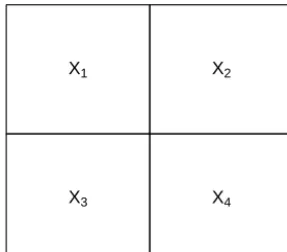
Figure 1.Graphical representation of a 2×2 lattice and elements ofx.

– reflects the kind of spatial dependency we assume our data has, and

– yields a legitimate covariance matrix,6, i.e. symmetric and positive definite, so that it can be used to compute a likelihood function.

Considerx, a vector of measurements on a 2×2 lattice, as represented in Fig. 1. Assume a neighborhood structure between the four elements ofx. In Fig. 2, the neighbors for each element ofx are defined graphically. Given the neigh-borhood structure shown in Fig. 2, the precision matrix that works for this problem is

Q=



  

2 −1 −1 0

−1 2 0 −1

−1 0 2 −1

0 −1 −1 2



  

,

which follows these rules:

– Qij= −1, ifxi andxjare neighbors.

– Qij=0, ifxiandxj are not neighbors.

– Qiigives the total number of neighbors ofxi.

While the implementation of GMRFs is simple, the theory and mathematics are rather involved. A more full descrip-tion of the mathematics of this example is provided in the Supplement. It may also not be immediately clear to a phys-ical scientist that such a simple specification, where only re-lationships among neighboring grid cells are taken into ac-count, would be sufficient to quantify correlated quantities across large distances. The mathematics of working with pre-cisions allows one to infer the net effect of long-distance rela-tionships through relationship information that exists among neighboring cells. While the GMRF approach does not in-clude information about particular teleconnection structures such as ENSO, the approach is sensitive to how changes in large-scale conditions induce local covariances across multi-ple fields within the entire domain. In this way teleconnec-tions are represented through a conditional dependence.

X1

X3

X2

X4

X1

X3

X2

X4

X1

X3

X2

X4

X1

X3

X2

X4

Figure 2.Neighbors ofx1, x2, x3andx4

A problem arises in that one of the eigenvalues of theQ matrix is 0, which implies that this definition of the preci-sion matrix does not induce an invertible covariance matrix. AlthoughQmay be inverted using the Moore–Penrose pseu-doinverse, we have solved this problem by usingαI+(1−

α)Q, instead ofQ. Ifαis small, the neighborhood structure remains essentially unchanged. Section 3 describes our ap-proach to specifying a value forα.

2.2 Generalizing concepts to deal with multiple fields The generalization ofQto handle multiple fields involves a Kronecker product (⊗) betweenS−1andQ. For reference, a Kronecker product ofA⊗Bwhere

A=

1 4 2 5

andB=

1 3 0 4

is given by

A⊗B=

1(B) 4(B)

2(B) 5(B)

=



  

1 3 4 12

0 4 0 16

2 6 5 15

0 8 0 20



  

.

Considerx and y which represent observations for two different fields of interest on a 2×2 lattice. First, x and y are combined to form one vector v as follows: vT =(x1, x2, x3, x4, y1, y2, y3, y4).The average covariances among these observations can be represented by a 2×2 ma-trix between the first field,x, and the second field,y:

S=

σ11 σ12

σ21 σ22

,

where Var(x)=σ11, Var(y)=σ22, and Cov(x,y)=σ12. Recalling that the correlation between fields 1 and 2 is de-fined asρ=_√σ12

(4)

0.0 0.2 0.4 0.6 0.8 1.0

0.6

0.8

1.0

1.2

α f(α)

Figure 3.αvs.f (α).

S−1=



  

1

σ11(1−ρ2)

−ρ

(1−ρ2₎√_σ

11σ22

−ρ

(1−ρ2₎√_σ

11σ22

1

σ22(1−ρ2)



  

=

S₁₁−1 S₁₂−1

S₂₁−1 S₂₂−1

.

If we consider the Kronecker product in Eq. (2) whenα=0,

S−1⊗Q=

S−₁₁1Q S₁₂−1Q

S−₂₁1Q S₂₂−1Q

,

then

vTS−1⊗Qv=S₁₁−1xTQx+S₁₂−1yTQx

+S₂₁−1xTQy+S₂₂−1yTQy.

In this last expression, one can see that the inverse of S in combination with the Kronecker product withQincludes terms involving cross products between fields. The Supple-ment carries this expression one step further by estimating the conditional mean for the first element ofv to illustrate how this element is related to itself and its neighbors across multiple fields.

3 A test of GMRF estimates of variance

GMRFs provide a way to approximate field and space de-pendencies contained in the inverse covariance matrix 6−1 of Eq. (1) by its GMRF equivalent S−1⊗(αI+(1−α)Q). In this section, we will test how well GMRFs are able to re-produce observed space and field dependencies. This may be achieved by comparing field and spatial variance and co-variance estimates obtained from the inverse of the GMRF

−4 −2 0 2 4

0.0

0.1

0.2

0.3

α =_0.0026

Empirical GMRF

−4 −2 0 2 4

0.0

0.1

0.2

0.3

α =₁

Distance Distance

Variance Variance

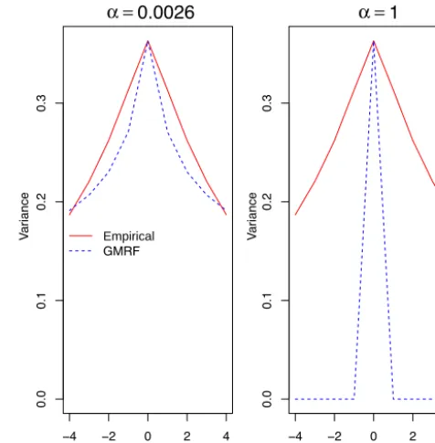
Figure 4.“Witch hat” graphs for air temperature on a 128×22 lat-tice of the tropics from 30◦S to 30◦N. The empirical estimates are given by the solid red line. The GMRF estimate is given by the dashed blue line.

Table 1.Correlation matrix between four fields from CAM 3.1.

PRECT PSL TREFHT U

PRECT 1 −0.219 −0.047 0.015

PSL −0.219 1 −0.313 −0.112

TREFHT −0.047 −0.313 1 −0.145

U 0.015 −0.112 −0.145 1

estimate of the precision matrix with those obtained empiri-cally from observational data. It turns out this comparison is sensitive to the value that is selected forα. By construction, the optimal choice ofαdepends only on geometric consider-ations of the neighborhood model that is used for GMRF and the number of grid points in the fields and not the properties of the field data. We introduce a “witch hat” graph that pro-vides a compact summary of variance–covariance informa-tion between these two methods in order to show that GM-RFs do a reasonable job approximating observed field and space relationships.

3.1 Finding an appropriate value ofα

In the effort to compare space and field dependencies ap-proximated by GMRF with empirical estimates we need to determine an optimal value for α. In order to carry out this comparison, we need to find the inverse ofS−1⊗

(5)

c0

0 1e4 2e4 3e4 4e4 5e4 6e4

2e−6 4e−6 6e−6 8e−6 1e−5 1e-3

2e-3 3e-3 4e-3 5e-3

Ke

(a) Field and space independence

0 1e4 2e4 3e4 4e4 5e4 6e4

2e−6 4e−6 6e−6 8e−6 1e−5 2e-3

3e-3 4e-3 5e-3

Ke

(b) Field dependencies

2e−6 4e−6 6e−6 8e−6 10e−6 1e-3

2e-3 3e-3 4e-3 5e-3

Ke

(c) Field and space dependencies

1e-3

0 2e4 4e4 6e4 8e4 10e4 12e4

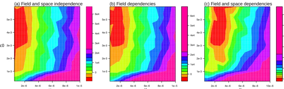
Figure 5.Three versions of the GMRF-based cost as a function of two CAM3.1 parameterskeandc0that assumes the data have(a)field and space independence, (b)field dependencies, and(c)field and space dependencies. Each color represents ten percentiles of the cost distribution. The cost is shown relative to the value of the default model configuration.

S−1⊗(αI+(1−α)Q)−1=S⊗(αI+(1−α)Q)−1. Letting Q∗=(αI+(1−α)Q)−1, thenS⊗Q∗for two fields can be written as

S11Q∗ S12Q∗

S21Q∗ S22Q∗

.

Ifnis the total number of grid points of the lattice,S⊗Q∗

is a 2n×2n covariance matrix. Note that each element of diag(SijQ∗)contains the estimated variance or covariance at

each grid point for fieldsiandjusing a GMRF whereican be equal toj. If we average these estimates across the whole lattice, we obtainGij, the GMRF estimate of the variance or

covariance for fieldsiandj. Therefore,

Gij=

SijPnk=1Q

∗ kk

n =

Sijtr(Q∗)

n , (3)

where tr(Q∗)denotes the trace ofQ∗andQ∗_kk are its diag-onal elements. We will now select a value for αthat allows the GMRF estimate for field variances and covariances to be equal, on average, to what has been calculated forS. In order to achieve this,Gijneeds to equalSij. Satisfying this

condi-tion is equivalent to finding the solucondi-tion for tr(Q∗₎

n =1. (4)

It may not be so obvious what the diagonal elements ofQ∗

are. However, one can use the fact that tr(A)is equal to the sum of its eigenvalues. In our case, if the eigenvalues ofQ

areλ1, λ2, . . ., λn, the eigenvalues ofαI+(1−α)Qareα+

(1−α)λ1, α+(1−α)λ2, . . ., α+(1−α)λn. The eigenvalues

ofQ∗=(αI+(1−α)Q)−1are(α+(1−α)λ1)−1, (α+(1−

α)λ2)−1, . . ., (α+(1−α)λn)−1. This implies that in order to

satisfy Eq. (4), we need to findαfrom

f (α)=

n X

i=1

1

n(α+(1−α)λi)

=1. (5)

Figure 3 shows the relationship between various values of

αandf (α). The eigenvalues used to obtain this figure

corre-spond to the precision operator,Q, for a GMRF induced by a first-order neighborhood structure and considering a 128×22 lattice (which is the dimension of our data). From the figure we can see that the curve crosses the value of 1 whenαis close to 0. By using linear interpolation, we determine that

αis approximately 0.0026. Note that this value is indepen-dent of fields since Eq. (5) does not contain any field-specific information.

3.2 “Witch hat” comparison test

To illustrate any differences that may exist between empirical estimates of the covariance matrix6and its GMRF equiva-lentS⊗(αI+(1−α)Q)−1, we rely on a graph that shows the spatial average grid point variance and covariances as a function of distance for cells and their neighbors. We com-pute the average entries of the covariance matrix correspond-ing to each grid cell and the correspondcorrespond-ing element to the north or east (for the positive distances) or to the south or west (for the negative distances) relative to the main diago-nal of the matrix. The zero distance case is the average of variances of the main diagonal. The cells corresponding to one or more grid cells away are mostly on entries in paral-lel with the main diagonal. On average, covariances decrease with distance, making the graph have the shape of a witch’s hat. This graph is symmetric because covariance matrices are symmetric.

(6)

Cost

2e−6 6e−6 1e−5

Ke 2e−6 6e−6Ke 1e−5 2e−6 6e−6Ke 1e−5

-10 000

0

10 000

20 000

30 000

40 000

-10 000

0

10 000

20 000

30 000

40 000

-10 000

0

10 000

20 000

30 000

40 000

TOTAL PSL TREFHT U PRECT

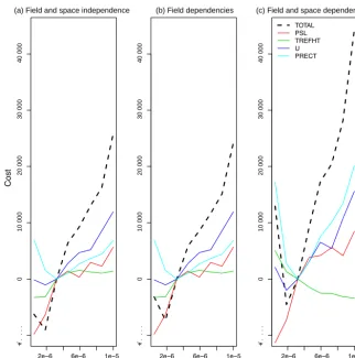
Figure 6.Different field contributions to the GMRF-based costs for a slice of Fig. 5 wherec0=0.0035. Cost values are relative to the default parameter setting for ke. Note that total cost (black dashed line) is a weighted sum of field contributions as given byS−1with contributions from sea level pressure (PSL, red line), 2 m air temperature (TREFHT, green line), 200-millibar zonal winds (U, blue line), and total precipitation (PRECT, cyan line).

other hand, whenα=0.0026, we allowQto play more of a role, which results in a better representation of covariances at neighboring points (lags different of zero).

4 Climate response to uncertain parameters

In this section we show how inclusion of field and space de-pendencies using GMRF affects comparisons of the Commu-nity Atmosphere Model (CAM3.1) (Collins et al., 2006) with observations. We consider CAM3.1’s response to changes in parameterke, which controls raindrop evaporation rates, and parameterc0, which controls precipitation efficiency through conversion of cloud water to rain water. For this comparison we only consider the response for the June, July, and August (JJA) seasonal mean between 30◦S and 30◦N on four vari-ables including 2 m air temperature (TREFHT), 200-millibar zonal winds (U), sea level pressure (PSL), and precipitation (PRECT). Experiments with CAM3.1 use observed clima-tological sea surface temperatures and sea ice extents. Each experiment with CAM3.1 is 32 years in duration.

The observational data that are used to evaluate the model come from a ECMWF-ERA interim reanalysis product (Up-pala et al., 2005) for 2 m air temperature, 200-millibar zonal winds, and sea level pressure and GPCP (Adler et al., 2009) for precipitation. We make use of approximately 30 years of JJA mean fields between 1979 and 2009. To construct S, we calculate variances from 2-year means (i.e., 15 samples).

(7)

The correlation matrix, R, corresponding to theSmatrix of 2-year JJA seasonal mean variances and covariances, as estimated from 30 years of observations, is shown in Table 1. The primary field correlations are the values of (−0.313) and (−0.219) occurring between sea level pressure (PSL) and 2 m air temperature (TREFHT), and precipitation (PRECT) and sea level pressure (PSL), respectively. Maps of the grid point correlations between these fields show a lot of struc-ture with regions of both positive and negative correlations. Therefore, providing a mechanistic explanation of the spa-tially averaged correlation is not particularly meaningful. De-spite losing regional information in theSmatrix summary of field covariances, GMRF estimated field covariances as seen within “witch hat” graphs are reasonable as compared to em-pirical estimates (see Supplement).

Figure 5 shows a comparison of the three versions of the GMRF-based cost for the 64 experiments within an 8×8 lattice. All versions of cost result in qualitatively similar re-sults with high and low cost values roughly in the same por-tions of parameter space. The main difference among the ver-sions of cost comes from taking space dependencies into ac-count within the field-space version. In this case, extremely low values ofkeresult in higher metric values. Figure 6 ex-amines the reasons for this by graphing the different field contributions to the GMRF-based costs for a slice where

c0=0.0035, which corresponds to one of the rows of the lat-tice. By plotting everything differenced from metric values at ke=3×10−6, one can learn that the biggest qualitative difference comes from cost values associated with 2 m air temperature. Closer inspection of differences between model output and observations of 2 m air temperature (not shown) indicates that the traditional cost is likely reflecting large-scale differences over the Southern Hemisphere oceans. In-clusion of space dependencies places much greater signifi-cance on smaller-scale anomalies occurring over the conti-nents, particularly over the Andes Mountains. This finding is a result of the mathematics of GMRF. It does not im-ply that the large-scale errors are of lesser scientific impor-tance. It only means that GMRFs are less sensitive to large-scale anomalies, perhaps because they are associated with fewer degrees of freedom than highly structured errors. Un-derstanding whether and how these distinctions aid model assessment needs further study. We do find it reassuring that GMRF-based metrics of distance to observations are similar, at least in the example provided, to a traditional metric.

5 Summary

We have developed a new test statistic as a scalar measure of model skill or cost for evaluating the extent to which cli-mate model output captures observed field and space rela-tionships using Gaussian Markov random fields (GMRFs). The challenge has been that few observations exist for es-tablishing a meaningful observational basis for quantifying

field and space relationships of climate phenomena. Much of the data that are typically used for model evaluation are sus-pected of having their own relationship biases introduced by the numerical model that is used to synthesize measurements into gridded products. The GMRF-based metric overcomes some of these limitations by considering field and space vari-ations within a neighborhood structure, thereby lowering the metric’s data requirements. The form of the metric separates space and field dependencies using a Kronecker product that, when multiplied out, has all the terms necessary to represent how different points in space are tied together across mul-tiple fields. We also include a scalarαthat weights the im-portance of spatial relationships between grid cells. Its opti-mal value turns out to be independent of the data type, which aids the use of GMRFs for comparing model output to data across multiple fields. Using “witch hat” graphs, we show a first-order (nearest neighborhood) structure does an excellent job of capturing empirical estimates of field and space rela-tionships for various lag windows or distances. We have ap-plied three versions of cost that selectively turn on or off field and space dependencies in a climate model (CAM3.1) output against observational products for tropical JJA climatologies for 2 m air temperature, sea level pressure, precipitation, and 200-millibar zonal winds. The results show subtle but poten-tially important differences among these versions of the cost which may prove beneficial for selecting models that capture observed climate phenomena for the right reasons.

6 Code and data availability

R code and data for generating Figs. 5 and 6 can be obtained through https://zenodo.org/record/33765 (Nosedal-Sanchez et al., 2015).

The Supplement related to this article is available online at doi:10.5194/gmd-9-2407-2016-supplement.

Acknowledgements. This material is based upon work supported

by the US Department of Energy Office of Science, Biolog-ical and Environmental Research Regional & Global Climate Modeling Program under award numbers DE-SC0006985 and DE-SC0010843. Alvaro Nosedal-Sanchez was partially supported by the National Council of Science and Technology of Mexico (CONACYT).

Edited by: P. Ullrich

(8)

Adler, R. F., Huffman, G. J., Chang, A., Ferraro, R., Xie, P.-P., Janowiak, J., Rudolf, B., Schneider, U., Curtis, S., Bolvin, D., Gruber, A., Susskind, J., Arkin, P., and Nelkin, E.: The Version-2 Global Precipitation Climatology Project (GPCP) Monthly Precipitation Analysis (1979– Present), J. Hydrometeorol., 1147–1167, doi:10.1175/1525-7541(2003)004<1147:TVGPCP>2.0.CO;2, 2009.

Braverman, A., Cressie, N., and Teixeira, J.: A likelihood-based comparison of temporal models for physical processes, Statis-tical Analysis and Data Mining, 4, 247–258, 2011.

Collins, W. D., Rasch, P. J., Boville, B. A., Hack, J. J., McCaa, J. R., Williamson, D. L., and Briegleb, B. P.: The formulation and atmospheric simulation of the Community Atmosphere Model version 3 (CAM3), J. Climate, 19, 2144–2161, 2006.

Cressie, N. and Wikle, C. K.: Statistics for Spatio-Temporal Data, Wiley, Hoboken, NJ, 2011.

Gleckler, P. J., Taylor, K. E., and Doutriaux, C.: Performance met-rics for climate models, J. Geophys. Res.-Atmos., 113, 1–20, 2008.

Knutti, R., Furrer, R., Tebaldi, C., Cermak, J., and Meehl, G. A.: Challenges in combining projections from multiple climate mod-els, J. Climate, 23, 2739–2758, 2010.

Nosedal-Sanchez, A., Jackson, C. S., and Huerta, G.: Code for “A new metric for climate models that includes field and spatial de-pendencies using Gaussian Markov Random Fields”, Zenodo, doi:10.5281/zenodo.33765, 2015.

Reichler, T. and Kim, J.: How Well Do Coupled Models Simulate Today’s Climate?, B. Am. Meteorol. Soc., 89, 303–311, 2008.

Santer, B. D., Taylor, K. E., Gleckler, P. J., Bonfils, C., Barnett, T. P., Pierce, D. W., Wigley, T. M. L., Mears, C., Wentz, F. J., Brügge-mann, W., Gillett, N. P., Klein, S. A., Solomon, S., Stott, P. A., and Wehner, M. F.: Incorporating model quality information in climate change detection and attribution studies, P. Natl. Acad. Sci. USA, 106, 14778–14783, 2009.

Taylor, K.: Summarizing multiple aspects of model performance in a single diagram, J. Geophys. Res.-Atmos., 106, 7183–7192, 2001.

Trenberth, K. E., Koike, T., and Onogi, K.: Progress and Prospects for Reanalysis for Weather and Climate, Eos T. Am. Geophys. Un., 89, 234–235, 2008.

Uppala, S. M., Kållberg, P. W., Simmons, A. J., Andrae, U., Bech-told, V. D. C., Fiorino, M., Gibson, J. K., Haseler, J., Hernandez, A., Kelly, G. A., Li, X., Onogi, K., Saarinen, S., Sokka, N., Al-lan, R. P., Andersson, E., Arpe, K., Balmaseda, M. A., Beljaars, A. C. M., Berg, L. V. D., Bidlot, J., Bormann, N., Caires, S., Chevallier, F., Dethof, A., Dragosavac, M., Fisher, M., Fuentes, M., Hagemann, S., Hólm, E., Hoskins, B. J., Isaksen, L., Janssen, P. A. E. M., Jenne, R., Mcnally, A. P., Mahfouf, J. F., Morcrette, J. J., Rayner, N. A., Saunders, R. W., Simon, P., Sterl, A., Tren-berth, K. E., Untch, A., Vasiljevic, D., Viterbo, P., and Woollen, J.: The ERA-40 re-analysis, Q. J. Roy. Meteor. Soc., 131, 2961– 3012, 2005.