Changes in regional climate extremes as a function of global mean temperature: an interactive plotting framework

(1)

https://doi.org/10.5194/gmd-10-3609-2017 © Author(s) 2017. This work is distributed under the Creative Commons Attribution 3.0 License.

Changes in regional climate extremes as a function of global

mean temperature: an interactive plotting framework

Richard Wartenburger1, Martin Hirschi1, Markus G. Donat2,3, Peter Greve4, Andy J. Pitman2,3, and Sonia I. Seneviratne1

1_{Institute for Atmospheric and Climate Science, ETH Zurich, Zurich, Switzerland}

2_{ARC Centre of Excellence for Climate System Science, University of New South Wales, Sydney, Australia} 3_{Climate Change Research Centre, University of New South Wales, Sydney, Australia}

4_{International Institute for Applied Systems Analysis (IIASA), Laxenburg, Austria}

Correspondence to:Richard Wartenburger ([email protected]) and Sonia I. Seneviratne ([email protected])

Received: 6 February 2017 – Discussion started: 21 February 2017

Revised: 27 June 2017 – Accepted: 19 August 2017 – Published: 29 September 2017

Abstract.This article extends a previous study (Seneviratne et al., 2016) to provide regional analyses of changes in cli-mate extremes as a function of projected changes in global mean temperature. We introduce the DROUGHT-HEAT Re-gional Climate Atlas, an interactive tool to analyse and dis-play a range of well-established climate extremes and water-cycle indices and their changes as a function of global warm-ing. These projections are based on simulations from the fifth phase of the Coupled Model Intercomparison Project (CMIP5). A selection of example results are presented here, but users can visualize specific indices of interest using the online tool. This implementation enables a direct assessment of regional climate changes associated with global mean tem-perature targets, such as the 2 and 1.5◦limits agreed within the 2015 Paris Agreement.

1 Introduction

The 2015 United Nations Climate Change Conference in Paris (COP21) recently set the goal of limiting global mean temperature increases to “well below 2 degrees” and to pur-sue efforts to limit warming to 1.5◦C above pre-industrial levels. Despite this global agreement, the implications of these global mean temperature thresholds have not been fully assessed. Specifically, stakeholders, decision-makers, and the public need more detailed information with respect to as-sociated changes on regional scales, in particular for extreme

events and impacts on humans and ecosystems (e.g. Senevi-ratne et al., 2016, hereafter S16; see also, e.g. Schleussner et al., 2016; Guiot and Cramer, 2016; James et al., 2017).

(2)

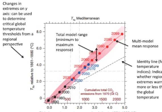
Figure 1.Example of a plot displaying the functional relationship of a regional climate index (annual maximum of daily maximum temper-ature,TXx) on global mean temperature following the S16 approach, including explanatory annotations (adapted from S16).

2014). However, this approach also allows to visually assess nonlinearities in the functional relationships.

We provide an illustration of the display used in S16 in Fig. 1. The main advantage of this approach is that it pro-vides, in a single figure, information on (a) the response of a given regional quantity for different global mean temper-ature (and greenhouse gas emissions) targets, (b) an empiri-cal assessment of this functional relationship (allowing, e.g. to identify its possible (non)linearity), and (c) the range of model and scenario response around this value. Hence, com-plex information can be more easily conveyed to regional stakeholders, instead of being summarized in several global analyses or provided as time- and scenario-dependent infor-mation. While globally aggregated information also has ob-vious value (e.g. O’Neill et al., 2017), regional information is of critical importance for adaptation and communication.

The S16 study, which focused on temperature and precip-itation extremes for two emissions scenarios (RCP8.5 and RCP4.5), identified that much of the absolute changes in tem-perature extremes and heavy precipitation events could be re-lated almost linearly to the changes in global mean tempera-ture for the time period 1860–2099 (see also Fig. 1), and that this functional relationship was very similar for the two dif-ferent emissions scenarios. In addition, it highlighted that – in absolute terms – changes in regional temperature extremes tended to be much larger than the global mean temperature change. The regional model spread was found to be highly variable depending on the considered quantity and region (S16). We note that all analyses focused on the transient cli-mate response and not on the response at clicli-mate equilibrium, which is expected to be substantially different. In addition, it does not consider aspects related to, e.g. overshooting of cli-mate targets or irreversibility in the clicli-mate response (Knutti

et al., 2016). Moreover, S16 considered changes in absolute temperature extremes and not in the probability of exceed-ing a given temperature threshold, which by design would tend to change exponentially when mean regional tempera-ture approaches the set threshold (e.g. Fischer and Knutti, 2015), even in the case of a linear relationship of the changes in absolute temperature extremes (Whan et al., 2015).

As a follow-up to the S16 study, we provide several new contributions and analyses. First, we introduce a new web-based interactive plotting framework (hereafter referred to as the DROUGHT-HEAT Regional Climate Atlas, available via http://www.drought-heat.ethz.ch/atlas) for the visualiza-tion of key funcvisualiza-tional relavisualiza-tionships on global mean temper-ature, so that the results can be easily shared with other re-searchers and stakeholders. The DROUGHT-HEAT Regional Climate Atlas has been augmented by several variables com-pared to the analyses of S16, including responses in regional mean temperature and precipitation and additional climate extremes. In addition, the analyses are performed for all four CMIP5 emissions scenarios (RCP2.6, RCP4.5, RCP6.0, and RCP8.5). These results can be assessed interactively by users online. An overview of the main functional relation-ships and a comparison with the previous analyses of S16 are discussed in Sect. 3.1. We provide some detailed anal-yses of specific features of interest for the interpretation of the results. In particular, we assess differences in regional re-sponses at 1.5, 2, and 3◦_{C global mean temperature increases}

(3)

2100 (Sect. 3.4) to assess the links between long-term vs. short-term responses.

2 Methods and data

This section presents the data sources and methods used to produce the DROUGHT-HEAT Regional Climate Atlas. It is structured as follows: Sect. 2.1 and 2.2 introduce the set of model simulations and climate and extremes indices which the analyses are based on. The S16 empirical global mean temperature relationship approach is presented in Sect. 2.3. Finally, Sect. 2.4 describes the content and technical imple-mentation of the DROUGHT-HEAT Regional Climate Atlas. 2.1 Model simulations

The presented regional-scale functional relationships be-tween a range of indices and global mean temperature are derived from global climate model (GCM) simulations from the Coupled Model Intercomparison Project Phase 5 (CMIP5; Taylor et al., 2012). The subset of GCMs used in this study includes all models for which (a) daily data are available within CMIP5 and (b) climate change indices from the joint CCl/CLIVAR/JCOMM Expert Team on Climate Change Detection and Indices (ETCCDI) are available (Sill-mann et al., 2013a, b).

To assess the impact of intra-model spread, we perform our analysis in two steps: using (a) only one ensemble mem-ber per model (r1i1p1) and (b) all memmem-bers available. Simi-lar to S16, we focus on model simulations over the time pe-riod 1861–2099, as this is the pepe-riod covered by virtually all models. For the evaluation of the functional relationship with global mean temperature beyond the end of the cen-tury, we also analyse a subset of simulations spanning all years from 1861 to 2299. For clarity of visual display, we ex-cluded model simulations of the RCP8.5 scenario for which no simulations exist in the historical period. To facilitate the calculation of regional ensemble averages, all GCM output has been bilinearly interpolated to a horizontal resolution of 2.5◦×2.5◦. The final set of model simulations employed in this study is listed in Table 1.

2.2 Climate and extremes indices

For the ensemble member e of each model m and emis-sion scenario rcpx, we have analysed the 27 ETCCDI core climate change indices Ircpx,m,e, which were downloaded

from the Canadian Centre for Climate Modelling and Anal-ysis (CCMA) indices archive (http://www.cccma.ec.gc.ca/ data/climdex/; Sillmann et al., 2013a, b) on 19 May 2016. Similar to the CMIP5 model data, the indices have been in-terpolated to 2.5◦×2.5◦horizontal resolution.

In addition to the ETCCDI indices, we have computed three drought indices (which can be used to monitor ei-ther anomalously dry or anomalously wet conditions) based

on soil moisture, precipitation, and evapotranspiration from CMIP5 model simulations (see Sect. 2.1) using the R sta-tistical language and the Climate Data Operators (CDO). The Standardized Precipitation Index (SPI) has been calcu-lated using the SPEI package (https://cran.r-project.org/web/ packages/SPEI, based on Vicente-Serrano et al., 2010) for an accumulation period of 12 months. Soil moisture anomalies (SMAs, given in units of standard deviations in order to be independent on model-specific parametrizations of soil mois-ture depths) have been derived according to the procedure used in Orlowsky and Seneviratne (2012, 2013), which in-cludes a posterior filtering of SMAs using a median absolute deviation filter. In addition, we provide analyses for changes in precipitation minus evapotranspiration (P−E) as a further measure of changes in land water availability (e.g. Greve and Seneviratne, 2015).

We also include mean temperature (T) and precipitation (P) in our analyses. We do this to assess whether the regional response of extremes is related to the regional mean climate response or rather reflects a specific behaviour of extremes in the regions examined. For simplicity, we also refer to these variables as indices. A complete list of all indices, their data source, and associated units is provided in Table 2.

2.3 Derivation of the functional relationship between changes in regional climate indices and global mean temperature

Yearly global mean temperaturesTglob,rcpx,m,e for emission

scenario rcpx have been derived from each ensemble mem-bereof modelm. BothIrcpx,m,eandTglob,rcpx,m,eare treated

as anomalies relative to the pre-industrial reference period of 1861–1880 (subscript ref). For all time stepst, we thus com-pute 1Tglob,rcpx,m,e,t=Tglob,rcpx,m,e,t−Tglob,rcpx,m,e,ref and

1Ircpx,m,e,t=Ircpx,m,e,t−Ircpx,m,e,ref. Note thatTglobrefers to a model estimate of past and projected future global mean near-surface temperatures which is known to be biased with respect to observation-based global mean temperature records that merge air temperatures over land and sea surface temperatures over the ocean (Cowtan et al., 2015).

We apply a common land–sea mask at 2.5◦×2.5◦to all indices as we focus on (extremes) indices that are mean-ingful over land. We then compute regionally averaged in-dices1Ireg,rcpx,m,e using the set of globally distributed

re-gions defined in Chap. 3 of the Special Report on Managing the Risks of Extreme Events and Disasters to Advance Cli-mate Change Adaptation (SREX; Seneviratne et al., 2012, Fig. 3-1 therein), hereafter referred to as SREX regions. We also average the indices over the additional regions defined in S16 as well as over global land (including ice sheets).

To test the significance of the functional relationship be-tween the regionally averaged indices and the global mean temperature signal, we apply an ordinary least squares fit be-tween1Tglob,rcpx,m,e and1Ireg,rcpx,m,e for each individual

(4)

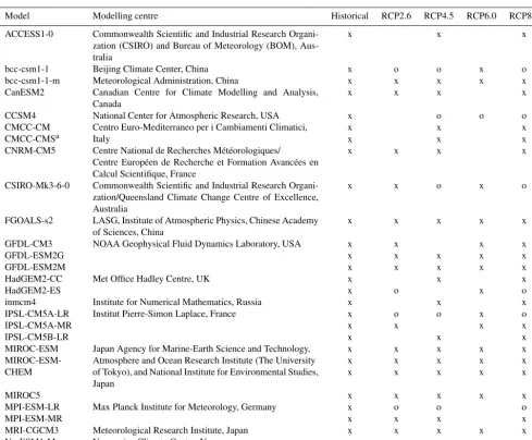
Table 1.List of models used in this study (in alphabetical order). Crosses (circles) indicate availability of simulations of the ensemble member r1i1p1 for the 1861–2099 (1861–2299) period. Note that the number of simulations of other ensemble members is considerably smaller.

Model Modelling centre Historical RCP2.6 RCP4.5 RCP6.0 RCP8.5

ACCESS1-0 Commonwealth Scientific and Industrial Research Organi-zation (CSIRO) and Bureau of Meteorology (BOM), Aus-tralia

x x x

bcc-csm1-1 Beijing Climate Center, China x o o x o

bcc-csm1-1-m Meteorological Administration, China x x x x x

CanESM2 Canadian Centre for Climate Modelling and Analysis, Canada

x x x x

CCSM4 National Center for Atmospheric Research, USA x o o o

CMCC-CM Centro Euro-Mediterraneo per i Cambiamenti Climatici, x x x

CMCC-CMSa Italy x x x

CNRM-CM5 Centre National de Recherches Météorologiques/

Centre Européen de Recherche et Formation Avancées en Calcul Scientifique, France

x x x x

CSIRO-Mk3-6-0 Commonwealth Scientific and Industrial Research Organi-zation/Queensland Climate Change Centre of Excellence, Australia

x x o x o

FGOALS-s2 LASG, Institute of Atmospheric Physics, Chinese Academy of Sciences, China

x x x x x

GFDL-CM3 NOAA Geophysical Fluid Dynamics Laboratory, USA x x x x

GFDL-ESM2G x x x x x

GFDL-ESM2M x x x x x

HadGEM2-CC Met Office Hadley Centre, UK x x x

HadGEM2-ES x o x o

inmcm4 Institute for Numerical Mathematics, Russia x x x

IPSL-CM5A-LR Institut Pierre-Simon Laplace, France x o o x o

IPSL-CM5A-MR x x x x

IPSL-CM5B-LR x x x

MIROC-ESM Japan Agency for Marine-Earth Science and Technology, x x x x x

MIROC-ESM- Atmosphere and Ocean Research Institute (The University x x x x x

CHEM of Tokyo), and National Institute for Environmental Studies, Japan

x x x x x

MIROC5 x x x x x

MPI-ESM-LR Max Planck Institute for Meteorology, Germany x o o o

MPI-ESM-MR x x x x

MRI-CGCM3 Meteorological Research Institute, Japan x x x x x

NorESM1-M Norwegian Climate Centre, Norway x x x x x

a_{Not used for calculation of}_P−E.

roughly represents future projections in the individual model simulations). The number of models for which the slope of the regression line (i.e. the measure of the functional rela-tionship) is significantly different from zero (p=0.01, after controlling the false discovery rate according to Benjamini and Hochberg, 1995, as recently suggested by Wilks, 2016) is used to indicate the robustness of the functional relation-ship in the ensemble mean of the changes (see Sect. 3). Note that a significant response of an individual model realization implies that the corresponding relationship can be explained by a linear model, though it does not guarantee superiority of the linear model over other, higher-order polynomials. We also test the significance of the differences of changes in be-tween 1.5 and 2◦C global warming based on all model simu-lations of a specific index and scenario, using a two-sided

paired Wilcoxon test (p=0.01, after controlling the false discovery rate according to Benjamini and Hochberg, 1995). To filter out short-term climatic fluctuations, a decadal running mean is applied to the anomalies, starting with 1871–1880 (note that the year associated with each run-ning mean period refers to the last year of that period). We then compute the unweighed ensemble mean change of the smoothed indices 1Ireg,rcpx=1Ireg,rcpx,m,e and the

corre-sponding ensemble mean change of the global mean temper-atures1Tglob,rcpx=1Tglob,rcpx,m,e.

In order to yield common, model-independent values of

1Tglob and to provide a bidirectional uncertainty estimate (i.e. including both the inter-model ensemble spread in

(5)

min-Table 2. List of indices (in alphabetical order) as presented in the DROUGHT-HEAT Regional Climate Atlas. Crosses denote indices specifically discussed in this paper as well as indices expressed as percent changes relative to the pre-industrial reference period (1861– 1880).

Index Description Unit Expressed as Discussed in Reference for computation

% change this paper

CDD Maximum length of dry spell days x Sillmann et al. (2013a, b)

CSDI Cold speel duration index days Sillmann et al. (2013a, b)

CWD Maximum length of wet spell days Sillmann et al. (2013a, b)

DTR Daily temperature range ◦C Sillmann et al. (2013a, b)

FD Number of frost days days Sillmann et al. (2013a, b)

GSL Growing season length days Sillmann et al. (2013a, b)

ID Number of icing days days Sillmann et al. (2013a, b)

P−E Precipitation – evapotranspiration mm day−1 x Greve and Seneviratne (2015)

P Mean precipitation mm x x Taylor et al. (2012)

PRCPTOT Annual total precipitation in wet days mm x Sillmann et al. (2013a, b)

R10mm Annual count of days when PRCP≥10 mm days Sillmann et al. (2013a, b)

R95pTOT Annual total PRCP when RR>95 % mm Sillmann et al. (2013a, b)

R99pTOT Annual total PRCP when RR>99 % mm Sillmann et al. (2013a, b)

Rx1day Monthly maximum 1-day precipitation mm x Sillmann et al. (2013a, b)

Rx5day Monthly maximum 5-day precipitation mm x x Sillmann et al. (2013a, b)

SDII Simple precipitation intensity index mm day−1 Sillmann et al. (2013a, b)

SMA Soil moisture anomalies 1 x Orlowsky and Seneviratne (2013)

SPI12 Standardized Precipitation Index (12-month accumulation period)

1 x Vicente-Serrano et al. (2010)

SU Number of summer days days Sillmann et al. (2013a, b)

T Mean temperature ◦C x Taylor et al. (2012)

TN10p Percentage of days whenT_N<10th percentile % days Sillmann et al. (2013a, b)

TN90p Percentage of days whenT_N>90th percentile % days Sillmann et al. (2013a, b)

TN n Monthly minimum of daily min. temperature ◦C x Sillmann et al. (2013a, b)

TN x Monthly maximum of daily min. temperature ◦C x Sillmann et al. (2013a, b)

TR Number of tropical nights days Sillmann et al. (2013a, b)

TX10p Percentage of days whenT_X<10th percentile % days Sillmann et al. (2013a, b)

TX90p Percentage of days whenT_X>90th percentile % days Sillmann et al. (2013a, b)

TXn Monthly minimum of daily max. temperature ◦C x Sillmann et al. (2013a, b)

TXx Monthly maximum of daily max. temperature ◦C x Sillmann et al. (2013a, b)

WSDI Warm spell duration index days Sillmann et al. (2013a, b)

imum and maximum of the interpolated values (across all model realizations and scenarios) are then used to determine the overall spread of1Iregrelative to1Tglob.

2.4 Plotting framework

2.4.1 Content of the plotting framework

All plots of the regional-scale functional relationships with global mean temperature and related figures similar to those shown in the remainder of this paper are available through the web interface of the DROUGHT-HEAT Regional Climate Atlas. All plots available through this interactive interface are based on the computation of the functional relationship with global mean temperature using the S16 framework as described in the previous section.

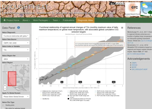
The layout and individual components of the DROUGHT-HEAT Regional Climate Atlas are shown in Fig. 2. Plots are

drawn by making the appropriate selections in the data panel (left-hand side of the screenshot). The first item to select is the diagnostic (i.e. “Functional relationship with global mean temperature” for the results of this study). After that, the data source drop-down menu is populated with a list of available data sets (i.e. CMIP5 model simulations for this study, for ei-ther the period 1861–2099 or 1861–2299). Equivalently, the drop-down menu labelled “Select Index or Variable” is filled with available indices. Credits of the selected diagnostic and data source are displayed on the right-hand panel.

(6)

Figure 2.Screenshot of the DROUGHT-HEAT Regional Climate Atlas. For demonstration, this screenshot displays the functional relation-ship of1T_Xxon1T_globbased on model simulations from 1861 to 2099 for the SREX region west North America (WNA).

in the map or by selecting a global domain), the requested plot is displayed in the main panel of the website. When the appropriate selections are made, a link appears allowing the user to navigate to a set of box plots showing the distribu-tion of the selected index for fixed global mean temperature targets of 1.5, 2 and 3◦C (for more details, see Sect. 3.2).

The atlas has been designed to be self-explanatory. Each item in the drop-down lists is accompanied by a short help text that shows up when hovering over it with the mouse. In addition, a pop-up window has been added to provide help for first-time users. Users interested in reusing the results shown in a specific plot can download the related data in comma-separated value (CSV) format.

2.4.2 Technical implementation of the plotting framework

The DROUGHT-HEAT Regional Climate Atlas is based on a number of web modules served through the Guni-corn web application server (http://guniGuni-corn.org/) and the

NGINX reverse-proxy server (https://www.nginx.com/). The website is built within the Django web framework (https: //www.djangoproject.com/). It is hosted on a web server at ETH Zurich.

The map shown in the data panel of the DROUGHT-HEAT Regional Climate Atlas (see Fig. 2) is based on Leaflet (http://leafletjs.com/). The background (world) layer is based on tilesets served via Mapbox (https://www.mapbox.com/). The region boundaries are read from text files in GeoJSON format.

(7)

(http://www.highcharts.com/) parses the input files to gener-ate the desired plot.

3 Results and discussion

In the following, we demonstrate the capabilities of the DROUGHT-HEAT Regional Climate Atlas by presenting some selected results. We also discuss some more in-depth analyses considering specific features of the assessed func-tional relationships between regional climate and global mean temperature changes.

3.1 Functional form of the relationship

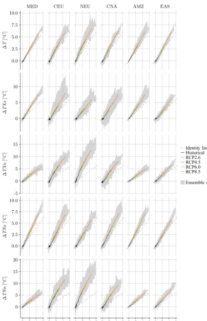
Figure 3 displays the relations of regional changes in temperature-based climate and extremes indices in various SREX regions to global mean temperature (1Tglob). The indices show an apparent linear scaling with 1Tglob when solely considering the ensemble mean change (the signifi-cance of the functional relationship of individual ensemble members is tested below; see Table 3). Moreover, the rela-tionship is apparently not influenced by differences in1Tglob among the model simulations (see Fig. A8 in the Appendix). As all indices in Fig. 3 are derived from temperatures, the scaling of changes in these indices shows similar linear fea-tures to the scaling of changes in regional mean temperafea-tures (1T, first row of Fig. 3). Besides this, the relationship of these indices to global mean temperature involves the least uncertainties (as measured by the ensemble spread) when compared to the other indices shown in Fig. 4. For all of the indicated regions, the slope of the temperature-based indices is consistently above 1 (although only by a small margin for

1TXnin the Amazon region, AMZ, which is also the case in

other tropical regions, not shown), indicating a larger change of the regional indices compared to1Tglob. For instance, at 2◦C global warming, the warming in hot extremes (TXx) in

the Mediterranean (SREX region MED) amounts to 3.2◦C. The largest departures from the identity line are found for changes in the annual minimum of both daily maximum and minimum temperatures (1TXn and1TN n) in north Europe

(NEU), which is very well in line with the observed recent decrease in temperature variance in the northern mid-to-high latitudes due to Arctic amplification (Screen, 2014).

For the precipitation-based indices discussed here, the responses are often less pronounced and subject to larger inter-model uncertainties (Fig. 4). Nevertheless, the ensem-ble mean changes of the purely precipitation-based indices (1P,1Rx5day,1CDD, and1SPI12) still show a distinct linear scaling with 1Tglob in some regions. For example, there is a clear tendency for a positive scaling of heavy pre-cipitation (1Rx5day) with1Tglob in NEU, central Europe (CEU), central North America (CNA), and east Asia (EAS). Moreover, MED displays a remarkable increase in the max-imum dry spell lengths (1CDD) by the end of the century

(i.e. the decade in which global mean temperature anoma-lies are projected to reach1Tglob=4.75◦C in the RCP8.5 scenario). This is consistent with the response of the drought indices (1SPI12, 1SMA, and 1P−E) in this region to-wards drying, although the large uncertainties in1SMA near the end of the century must not be ignored. The trends in

1SPI12,1SMA, and1P−Ein AMZ point towards a dry-ing in this region, which is unique among other tropical re-gions (not shown). However, it must be noted that – apart from the positive scaling of1SPI12 in NEU and EAS and the wetting signal indicated by1P−Ein NEU – the responses are connected with large uncertainties and both an increase and a decrease of these indices is within the projected range even for large values of1Tglob. Note that the differences be-tween the scaling of mean precipitation and heavy precipita-tion could possibly be explained by different sensitivities to aerosol loading (Pendergrass et al., 2015).

Overall, the functional relationship is very similar for the four emission scenarios (Figs. 3 and 4). Thus, regional changes in the indicated indices can be usefully related to given cumulative CO2 targets (according to S16), indepen-dently of the emission pathway.

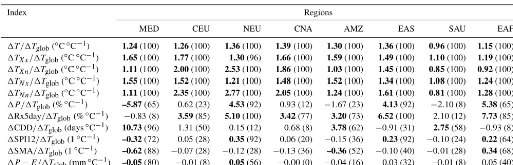
Table 3 displays the significant linear trends of the previ-ously discussed indices of the RCP8.5 scenario for1Tglob≥ 1◦C. Models generally agree that changes in global mean temperatures translate into enhanced changes both in re-gional mean temperatures over land as well as in rere-gional temperature extremes. The scaling with precipitation-derived indices shows a much more diverse pattern. Heavy precipi-tation events (as reflected by Rx5day) are projected to in-tensify over several of the selected regions, most strikingly over NEU, EAS, and EAF (east Africa). Dry spells are pro-jected to become longer mainly over MED and AMZ, which is in line with both a decrease in precipitation and enhanced soil moisture depletion as shown by1SMA (although pro-jections of CDD are generally dominated by larger uncertain-ties, which is in part due to high model sensitivities related to the binary cut-off of 1 mm used to distinguish dry days from days with precipitation). The Mediterranean region (MED) is the only region for which all relevant indices point towards a distinct drying. In contrast, precipitation is projected to in-crease with increasing global mean temperatures over NEU, EAS, and EAF. While this signal is consistent with the trend in SPI12 in each of the three regions, soil moisture anomalies are projected to only increase in EAF. Apart from MED, the model agreement on trends inP−Eis mostly poor.

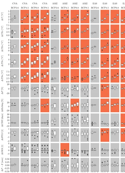
3.2 1.5 vs. 2◦C response

(8)

MED CEU NEU CNA AMZ EAS

0.0 2.5 5.0 7.5 10.0

0 5 10

-5 0 5 10 15

0.0 2.5 5.0 7.5 10.0

0 5 10 15 20

T

TXx

TXn

TNx

TNn

0 2 4 6 0 2 4 6 0 2 4 6 0 2 4 6 0 2 4 6 0 2 4 6

Identity line Historical RCP2.6 RCP4.5 RCP6.0 RCP8.5

Ensemble spread

(9)

-50 -25 0 25

-20 0 20 40

0 25 50 75 100

-2 0 2

-10 -5 0 5

-0.5 0.0 0.5 1.0

P

%

Rx5day

%

CDD

da

ys

SPI12

SMA

P

E

0 2 4 6 0 2 4 6 0 2 4 6 0 2 4 6 0 2 4 6 0 2 4 6

Ensemble spread

Historical RCP2.6 RCP4.5 RCP6.0 RCP8.5

(10)

MED RCP2.6

MED RCP4.5

MED RCP6.0

MED RCP8.5

CEU RCP2.6

CEU RCP4.5

CEU RCP6.0

CEU RCP8.5

NEU RCP2.6

NEU RCP4.5

NEU RCP6.0

NEU RCP8.5

2 4 6

0.0 2.5 5.0 7.5

5 10

0 2 4 6

5 10 15

-40 -20 0 20

-20 -100 10 20

0 40 80 120

-1 0 1 2

-7.5 -5.0 -2.50.0 2.5 5.0

-0.250.00 0.25 0.50

T

TXx

TXn

TNx

TNn

P

%

Rx5day

%

CDD

da

ys

SPI12

SMA

P

E

1.5 2 3 1.5 2 3 1.5 2 3 1.5 2 3 1.5 2 3 1.5 2 3 1.5 2 3 1.5 2 3 1.5 2 3 1.5 2 3 1.5 2 3 1.5 2 3

No signiﬁcant diﬀerence in between the distributions of for and

igniﬁcant diﬀerence in between the distributions of for and

S

(11)

CNA RCP2.6

CNA RCP4.5

CNA RCP6.0

CNA RCP8.5

AMZ RCP2.6

AMZ RCP4.5

AMZ RCP6.0

AMZ RCP8.5

EAS RCP2.6

EAS RCP4.5

EAS RCP6.0

EAS RCP8.5

1 2 3 4 5

0.0 2.5 5.0 7.5

0 2 4 6 8

2 4 6

0.0 2.5 5.0 7.5

-20 0 20

-100

10 20 30

-2 -1 0 1

-4 0 4 8

-0.50 -0.25 0.00 0.25 0.50

T

TXx

TXn

TNx

TNn

P

%

Rx5day

%

CDD

da

ys

SPI12

SMA

P

E

1.5 2 3 1.5 2 3 1.5 2 3 1.5 2 3 1.5 2 3 1.5 2 3 1.5 2 3 1.5 2 3 1.5 2 3 1.5 2 3 1.5 2 3 1.5 2 3

o signiﬁcant diﬀerence in between the distributions of for and

N S

(12)

Table 3.Scaling slopes of the RCP8.5 scenario for1Tglob≥1◦C and percent of models with a statistically significant linear scaling (in

brackets,p=0.01) for various SREX regions, based on CMIP5 simulations of ensemble member r1i1p1. Bold values indicate significance for at least 50 % of the contributing models for which the sign of the trend is identical to the sign of the ensemble mean trend. See Table 2 for a description of the indices.

Index Regions

MED CEU NEU CNA AMZ EAS SAU EAF

1T /1T_glob(◦C◦C−1) 1.24(100) 1.26(100) 1.36(100) 1.39(100) 1.30(100) 1.36(100) 0.96(100) 1.15(100) 1TXx/1Tglob(◦C◦C−1) 1.65(100) 1.77(100) 1.30(96) 1.66(100) 1.59(100) 1.49(100) 1.10(100) 1.19(100) 1TXn/1Tglob(◦C◦C−1) 1.11(100) 2.00(100) 2.53(100) 1.86(100) 1.03(100) 1.45(100) 0.85(100) 0.92(100) 1TN x/1Tglob(◦C◦C−1) 1.55(100) 1.52(100) 1.21(100) 1.48(100) 1.52(100) 1.34(100) 1.08(100) 1.24(100) 1TN n/1Tglob(◦C◦C−1) 1.11(100) 2.35(100) 2.77(100) 2.05(100) 1.24(100) 1.61(100) 0.81(100) 1.28(100) 1P /1T_glob(%◦C−1) –5.87(65) 0.62 (23) 4.53(92) 0.93 (12) −1.67 (23) 4.13(92) −2.10 (8) 5.38(65) 1Rx5day/1T_glob(%◦C−1) −0.83 (8) 3.59(85) 5.10(100) 3.42(77) 3.20(73) 6.52(100) 2.10 (12) 7.73(85) 1CDD/1T_glob(days◦C−1) 10.73(96) 1.31 (50) 0.15 (12) 0.68 (8) 3.78(62) −0.91 (31) 2.75(58) −0.93 (8) 1SPI12/1T_glob(1◦C−1) –0.32(72) 0.05 (28) 0.35(92) 0.06 (20) −0.15 (36) 0.23(92) −0.10 (24) 0.22(64) 1SMA/1T_glob(1◦C−1) –0.62(88) −0.07 (28) −0.12 (28) −0.13 (36) –0.36(52) −0.10 (40) −0.01 (28) 0.34(68) 1P−E/1T_glob(mm◦C−1) –0.05(80) −0.01 (8) 0.05(56) −0.00 (0) −0.04 (16) 0.03 (32) −0.01 (8) 0.05 (40)

are observable for virtually all of the temperature-based in-dices, when excluding the RCP2.6 scenario (where only 6 out of 18 models reach 1Tglob=2◦C). These findings are mostly independent from the Representative Concentra-tion Pathway (RCP) scenario chosen. For the precipitaConcentra-tion- precipitation-based indices, the differences in the response between the two global mean temperature targets are mostly insignificant. MED is projected to experience the strongest drying, as in-dicated by the significant increase in 1CDD (RCP4.5 and RCP8.5) and the corresponding decrease in water availabil-ity, as reflected by the decrease in1SMA (RCP8.5) and a de-crease in 1P−E (RCP4.5), confirming that this region is a potential hotspot for future drought-related changes (Or-lowsky and Seneviratne, 2013; Guiot and Cramer, 2016; Schleussner et al., 2016). On the other hand, NEU and EAS (Fig. 6) experience a significant increase in wet extremes. The other non-temperature indices show mostly no statis-tically significant distinction in the response between the two global mean temperature targets. The large spread in the precipitation-based indices in AMZ indicates that pre-cipitation projections in this region are subject to substan-tial uncertainties. The number of significant results for the precipitation-based indices shows some dependency on the scenario, with a slight dominance of significant differences in the RCP8.5 scenario.

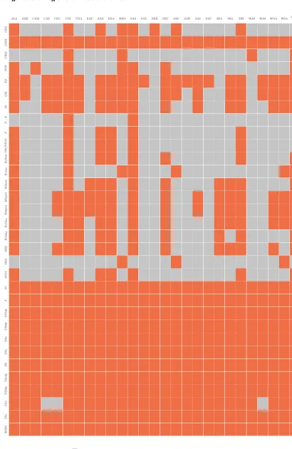
A broader overview of the significance in differences be-tween 1.5 and 2◦C global warming (using the same approach as above) considering all ETCCDI indices and SREX regions is provided in Fig. 7. Note that we focus on the RCP8.5 sce-nario here, as (1) the simulations of this scesce-nario all reach the 2◦global warming level and (2) this scenario constitutes the largest ensemble of simulations (see Fig. A8). There is an obvious dominance in significant differences for virtually all of the temperature related indices except from FD (frost

days), GSL (growing season length), and ID (icing days), for which the changes are (nearly) zero in all (sub)tropical re-gions. Precipitation changes are mostly significant in mid- to high-latitude regions, as reflected by the various related in-dices. The drought indices (P−E, SMA, and SPI12) show significant changes only in a few regions, either pointing to-wards a distinct wetting (e.g. SPI12 in east North America – ENA) or drying (e.g. SMA in south Africa – SAF).

3.3 Intra-model variability

The functional relationships and uncertainty ranges dis-cussed so far are based on one ensemble member (r1i1p1) of the applied models (see Table 1). In order to investigate any impact of intra-model variability on this range, Fig. 8 displays the ensemble mean and uncertainty ranges based on all ensemble members available for each model vs. the one-member-based ensemble mean and uncertainty range on the example of the precipitation-based indices discussed ear-lier. The regional signal of the functional relationship of

(13)

ALA AMZ CAM CAS CEU CGI CNA EAF EAS ENA MED NAS NAU NEB NEU SAF SAH SAS SAU SEA SSA TIB WAF WAS WNA WSA Global_and

CDD

CSDI

CWD

DTR

FD

GSL

ID

P

E

P

PRCPTOT

R10mm

R1mm

R20mm

R95ptot

R99ptot

Rx1day

Rx5day

SDII

SMA

SPI12

SU

T

TN10p

TN90p

TNn

TNx

TR

TX10p

TX90p

TXn

TXx

WSDI

N S

l

Figure 7.Significance of differences of1Iregin between the 1.5 and 2◦C global mean temperature targets based on mean temperatureT,

(14)

MED CEU NEU

-50 -25 0 25

-40 -20 0 20 40

-250 25 50 75 100

-2 0 2

-5 0 5 10

0.0 0.5 1.0

P

%

Rx5day

%

CDD

da

ys

SPI12

SMA

P

E

0 2 4 6 0 2 4 6 0 2 4 6

All members ens. mean r1i1p1 ens. mean

All members ens. spread r1i1p1 ens. spread

Figure 8.Functional relationships with global mean temperature for the indices1P,1Rx5day,1CDD,1SPI12,1SMA, and1P−E, averaged over the SREX regions MED, CEU, and NEU. Indices based on all CMIP5 ensemble members available per model (solid lines, dark shading) are compared with indices based on ensemble member r1i1p1 of each model (dashed lines, light shading). Values for1CDD> 100 days and1SMA<−5 were cut off for readability.

3.4 Beyond 2100

While most CMIP5 model simulations end by the end of the 21st century, a few simulations are available up to the year 2299 (see Table 1). These allow us to analyse the functional relationship beyond 2100 and to assess their longer-term be-haviour.

The long-term functional relationship of changes in temperature-related indices to changes in global mean tem-perature is similar (i.e. mostly linear in the ensemble mean) to the one shown in Fig. 3 (not shown). For the other indices,

(15)

-40 0 40

0 50 100

0 50 100 150 200

-6 -3 0 3

-8 -4 0

-0.5 0.0 0.5 1.0

P

%

Rx5day

%

CDD

da

ys

SPI12

SMA

P

E

0 5 10 15 0 5 10 15 0 5 10 15 0 5 10 15 0 5 10 15 0 5 10 15

Ensemble spread

(16)

short (1Rx5day) and longer-term (1SPI12) timescales. Ir-respective of the changes in1P,1Rx5day continues to in-crease in a near-linear fashion in all regions except MED.

4 Conclusions

We have developed the “DROUGHT-HEAT Regional Cli-mate Atlas”, a new interactive web interface available via http://www.drought-heat.ethz.ch/atlas, which provides plots of the functional relationship between changes in regional climate indices and global mean temperature for 26 larger IPCC predefined regions. Besides acting as a platform to fos-ter scientific discussion, the aim of this web infos-terface is to in-crease the accessibility of peer-reviewed scientific results to the general public, which is of major concern for the commu-nication of climate science findings (e.g. Harold et al., 2016). This is particularly relevant for the critical evaluation of the regional-scale implications of considered global mean tem-perature limits, such as the 1.5 and 2◦C temperature goals established in the 2015 Paris Agreement.

With the selected results presented here, we have demon-strated that a number of regionally averaged climate indices show a distinct linear relationship with global mean temper-atures both in the ensemble mean and in individual CMIP5 model realizations, as also illustrated in S16 for a more lim-ited set of indices and emissions scenarios. The linear rela-tionship is particularly obvious for the analysed temperature-derived indices and still present for a number of drought and water-cycle indices. We note, however, that some analyses display departures from such linear relationships, in partic-ular in the case of indices showing a low signal to noise in projections (e.g. in several regions for mean precipita-tion, dry spell lengths, soil moisture anomalies, and precip-itation minus evapotranspiration). Such departures are gen-erally more pronounced in the RCP2.6 scenario, because of the weak overall forcing in that emission scenario, and possi-bly also because of differences in aerosol forcing in RCP2.6 compared to the other emission scenarios (Pendergrass et al., 2015). These cases of non linearities illustrate the advantage of the applied S16 approach compared to traditional pattern scaling approaches, as the derived functional relationships are purely empirical and not assessed from a priori deter-mined mathematical relationships.

Projected changes in the indices are overall larger in a 2◦C world (i.e. 1Tglob=2◦C relative to pre-industrial levels) compared to a 1.5◦_{C world (i.e.}_1T

glob=1.5◦C relative to pre-industrial levels). The differences between the two global mean temperature limits are particularly large and generally significant for regional mean and extreme temperatures. Re-sults tend to be less robust for water-cycle indices, in par-ticular for those related to water availability (soil moisture anomalies or precipitation minus evapotranspiration). We en-courage the reader to use the DROUGHT-HEAT Regional Climate Atlas to evaluate these regional functional relation-ships using other indices or other regions than those pre-sented in this study.

The DROUGHT-HEAT Regional Climate Atlas has been designed to be easily expanded both in terms of functionality (e.g. adding support for additional plot types) and in terms of the number and type of supported data sets and diagnos-tics. By these means, we facilitate an easy extension of the platform to include graphical material from upcoming pub-lications within the scope of the DROUGHT-HEAT project and beyond.

Code availability. All code used to prepare the results discussed within this study is available upon request from the first author.

(17)

Appendix A: Supplementary figures

ALA RCP2.6

ALA RCP4.5

ALA RCP6.0

ALA RCP8.5

CAM RCP2.6

CAM RCP4.5

CAM RCP6.0

CAM RCP8.5

CAS RCP2.6

CAS RCP4.5

CAS RCP6.0

CAS RCP8.5

2 4 6 8

0.0 2.5 5.0

0 5 10 15

1 2 3 4 5

0 5 10 15

-20 0 20 40

-100

10 20 30

-2

-10

1 2 3

-5 0 5

-0.50

-0.250.00

0.25 0.50

T

TXx

TXn

TNx

TNn

P

%

Rx5day

%

CDD

da

ys

SPI12

SMA

P

E

1.5 2 3 1.5 2 3 1.5 2 3 1.5 2 3 1.5 2 3 1.5 2 3 1.5 2 3 1.5 2 3 1.5 2 3 1.5 2 3 1.5 2 3 1.5 2 3

N S

(18)

CGI RCP2.6

CGI RCP4.5

CGI RCP6.0

CGI RCP8.5

EAF RCP2.6

EAF RCP4.5

EAF RCP6.0

EAF RCP8.5

ENA RCP2.6

ENA RCP4.5

ENA RCP6.0

ENA RCP8.5

2 4 6

0 2 4 6

2.5 5.0 7.5 10.0 12.5

1 2 3 4 5

2.5 5.0 7.5 10.0 12.5

-100 10 20 30 40

-20 0 20 40

-10 0 10 20

0 1 2

-10 -5 0 5

0.0 0.4 0.8

T

TXx

TXn

TNx

TNn

P

%

Rx5day

%

CDD

da

ys

SPI12

SMA

P

E

1.5 2 3 1.5 2 3 1.5 2 3 1.5 2 3 1.5 2 3 1.5 2 3 1.5 2 3 1.5 2 3 1.5 2 3 1.5 2 3 1.5 2 3 1.5 2 3

o significant difference in between the distributions of for and ignificant difference in between the distributions of for and N

S

(19)

NAS RCP2.6

NAS RCP4.5

NAS RCP6.0

NAS RCP8.5

NAU RCP2.6

NAU RCP4.5

NAU RCP6.0

NAU RCP8.5

NEB RCP2.6

NEB RCP4.5

NEB RCP6.0

NEB RCP8.5

2 4 6

-2.50.0

2.5 5.0

0.0 2.5 5.0 7.5 10.0 12.5

1 2 3 4 5

2.5 5.0 7.5 10.0 12.5

-40

-200

20 40

-20 0 20 40

-100

10 20 30 40

-1 0 1 2

-5.0

-2.50.0

2.5 5.0

-0.5 0.0 0.5

T

TXx

TXn

TNx

TNn

P

%

Rx5day

%

CDD

da

ys

SPI12

SMA

P

E

1.5 2 3 1.5 2 3 1.5 2 3 1.5 2 3 1.5 2 3 1.5 2 3 1.5 2 3 1.5 2 3 1.5 2 3 1.5 2 3 1.5 2 3 1.5 2 3

N S

(20)

SAF RCP2.6

SAF RCP4.5

SAF RCP6.0

SAF RCP8.5

SAH RCP2.6

SAH RCP4.5

SAH RCP6.0

SAH RCP8.5

SAS RCP2.6

SAS RCP4.5

SAS RCP6.0

SAS RCP8.5

2 3 4

0 2 4 6

1 2 3 4

2 3 4 5

2 4 6

-50 0 50 100

0 400 800

-1 0 1

-10-5 0 5 10

0.0 0.4 0.8

T

TXx

TXn

TNx

TNn

P

%

Rx5day

%

CDD

da

ys

SPI12

SMA

P

E

1.5 2 3 1.5 2 3 1.5 2 3 1.5 2 3 1.5 2 3 1.5 2 3 1.5 2 3 1.5 2 3 1.5 2 3 1.5 2 3 1.5 2 3 1.5 2 3

S

(21)

SAU RCP2.6

SAU RCP4.5

SAU RCP6.0

SAU RCP8.5

SEA RCP2.6

SEA RCP4.5

SEA RCP6.0

SEA RCP8.5

SSA RCP2.6

SSA RCP4.5

SSA RCP6.0

SSA RCP8.5

1 2 3 4

1 2 3 4 5

0 1 2 3 4

1 2 3 4

-20 0 20 40

0 25 50

-10 0 10 20 30

-1.0 -0.50.0 0.5 1.0 1.5

-10-5 0 5 10

-0.5 0.0 0.5 1.0

T

TXx

TXn

TNx

TNn

P

%

Rx5day

%

CDD

da

ys

SPI12

SMA

P

E

1.5 2 3 1.5 2 3 1.5 2 3 1.5 2 3 1.5 2 3 1.5 2 3 1.5 2 3 1.5 2 3 1.5 2 3 1.5 2 3 1.5 2 3 1.5 2 3

o significant difference in between the distributions of for and ignificant difference in between the distributions of for and

N S

(22)

TIB RCP2.6

TIB RCP4.5

TIB RCP6.0

TIB RCP8.5

WAF RCP2.6

WAF RCP4.5

WAF RCP6.0

WAF RCP8.5

WAS RCP2.6

WAS RCP4.5

WAS RCP6.0

WAS RCP8.5

2 3 4 5

0 2 4 6

0.0 2.5 5.0

1 2 3 4 5

0 2 4 6

-30 0 30 60

-200 20 40 60

-500 50 100 150 200

-1 0 1 2

-4 -20 2 4 6

-0.3 0.0 0.3 0.6

T

TXx

TXn

TNx

TNn

P

%

Rx5day

%

CDD

da

ys

SPI12

SMA

P

E

1.5 2 3 1.5 2 3 1.5 2 3 1.5 2 3 1.5 2 3 1.5 2 3 1.5 2 3 1.5 2 3 1.5 2 3 1.5 2 3 1.5 2 3 1.5 2 3

S

(23)

WNA

RCP2.6 WNA

RCP4.5 WNA

RCP6.0 WNA

RCP8.5 WSA

RCP2.6 WSA

RCP4.5 WSA

RCP6.0 WSA

RCP8.5 Global

and RCP2.6

Global and RCP4.5

Global and RCP6.0

Global and RCP8.5

T

TXx

TXn

TNx

TNn

P

%

Rx5day

%

CDD

da

ys

SPI12

SMA

P

E

1.5 2 3 1.5 2 3 1.5 2 3 1.5 2 3 1.5 2 3 1.5 2 3 1.5 2 3 1.5 2 3 1.5 2 3 1.5 2 3 1.5 2 3 1.5 2 3 2

3 4

1 2 3 4 5 6

0.0 2.5 5.0 7.5

1 2 3 4 5

0 3 6 9

-10 0 10 20

0 10 20 30

0 20 40

-1.0 -0.5 0.0 0.5 1.0

-2.5 0.0 2.5

-0.25 0.00 0.25 0.50

o significant difference in between the distributions of for and ignificant difference in between the distributions of for and

l l l l

N S

(24)

1861–2099 1861–2299

r1i1p1

only

All

mem

bers

0 2 4 6 0 5 10 15

0 20 40 60 80

0 50 100 150

Num

ber

of

mo

del

sim

ulations

All scenarios

(25)

Competing interests. The authors declare that they have no conflict of interest.

Acknowledgements. R. Wartenburger and S. I. Seneviratne acknowledge the European Research Council (ERC) “DROUGHT-HEAT” project funded by the European Community’s Seventh Framework Programme (grant agreement FP7-IDEAS-ERC-617518). This study contributes to the World Climate Research Programme (WCRP) Grand Challenge on Extremes. We acknowl-edge the World Climate Research Programme’s Working Group on Coupled Modelling, which is responsible for CMIP, and we thank the climate modelling groups (listed in Table 1 of this paper) for producing and making available their model output. For CMIP, the US Department of Energy’s Program for Climate Model Diagnosis and Intercomparison provides coordinating support and led development of software infrastructure in partner-ship with the Global Organization for Earth System Science Portals.

Edited by: Richard Neale

Reviewed by: Ben Sanderson and one anonymous referee

References

Benjamini, Y. and Hochberg, Y.: Controlling the false discovery rate: a practical and powerful approach to multiple testing, J. R. Stat. Soc., 57, 289–300, 1995.

Cowtan, K., Hausfather, Z., Hawkins, E., Jacobs, P., Mann, M. E., Miller, S. K., Steinman, B. A., Stolpe, M. B., and Way, R. G.: Robust comparison of climate models with observations using blended land air and ocean sea sur-face temperatures, Geophys. Res. Lett., 42, 2015GL064888, https://doi.org/10.1002/2015GL064888, 2015.

Fischer, E. M. and Knutti, R.: Anthropogenic contribution to global occurrence of heavy-precipitation and high-temperature extremes, Nat. Clim. Change, 5, 560–564, https://doi.org/10.1038/nclimate2617, 2015.

Fischer, E. M., Sedlacek, J., Hawkins, E., and Knutti, R.: Mod-els agree on forced response pattern of precipitation and tem-perature extremes, Geophys. Res. Lett., 41, 2014GL062018, https://doi.org/10.1002/2014GL062018, 2014.

Frieler, K., Meinshausen, M., Mengel, M., Braun, N., and Hare, W.: A scaling approach to probabilistic assessment of regional climate change, J. Climate, 25, 3117–3144, https://doi.org/10.1175/JCLI-D-11-00199.1, 2012.

Greve, P. and Seneviratne, S. I.: Assessment of future changes in water availability and aridity, Geophys. Res. Lett., 42, 5493– 5499, https://doi.org/10.1002/2015GL064127, 2015.

Guiot, J. and Cramer, W.: Climate change: The 2015 Paris Agree-ment thresholds and Mediterranean basin ecosystems, Science, 354, 465–468, https://doi.org/10.1126/science.aah5015, 2016. Harold, J., Lorenzoni, I., Shipley, T. F., and Coventry, K. R.:

Cog-nitive and psychological science insights to improve climate change data visualization, Nat. Clim. Change, 6, 1080–1089, https://doi.org/10.1038/nclimate3162, 2016.

Huntingford, C. and Cox, P. M.: An analogue model to derive additional climate change scenarios from

ex-isting GCM simulations, Clim. Dynam., 16, 575–586, https://doi.org/10.1007/s003820000067, 2000.

James, R., Washington, R., Schleussner, C.-F., Rogelj, J., and Conway, D.: Characterizing half-a-degree difference: a re-view of methods for identifying regional climate responses to global warming targets, WIRES Clim. Change, 8, e457, https://doi.org/10.1002/wcc.457, 2017.

Knutti, R., Rogelj, J., Sedlacek, J., and Fischer, E. M.: A scientific critique of the two-degree climate change target, Nat. Geosci., 9, 13–18, https://doi.org/10.1038/ngeo2595, 2016.

Kravitz, B., Lynch, C., Hartin, C., and Bond-Lamberty, B.: Explor-ing precipitation pattern scalExplor-ing methodologies and robustness among CMIP5 models, Geosci. Model Dev., 10, 1889–1902, https://doi.org/10.5194/gmd-10-1889-2017, 2017.

Lopez, A., Suckling, E. B., and Smith, L. A.: Robustness of pattern scaled climate change scenarios for adaptation decision support, Climatic Change, 122, 555–566, https://doi.org/10.1007/s10584-013-1022-y, 2014.

Lynch, C., Hartin, C., Bond-Lamberty, B., and Kravitz, B.: Ex-ploring global surface temperature pattern scaling methodologies and assumptions from a CMIP5 model ensemble, Geosci. Model Dev. Discuss., https://doi.org/10.5194/gmd-2016-170, 2016. Mitchell, T. D.: Pattern scaling: an examination of the accuracy of

the technique for describing future climates, Climatic Change, 60, 217–242, https://doi.org/10.1023/A:1026035305597, 2003. O’Neill, B. C., Oppenheimer, M., Warren, R., Hallegatte, S., Kopp,

R. E., Pörtner, H. O., Scholes, R., Birkmann, J., Foden, W., Licker, R., Mach, K. J., Marbaix, P., Mastrandrea, M. D., Price, J., Takahashi, K., van Ypersele, J.-P., and Yohe, G.: IPCC reasons for concern regarding climate change risks, Nat. Clim. Change, 7, 28–37, https://doi.org/10.1038/nclimate3179, 2017.

Orlowsky, B. and Seneviratne, S.: Global changes in extreme events: regional and seasonal dimension, Climatic Change, 110, 669–696, https://doi.org/10.1007/s10584-011-0122-9, 2012. Orlowsky, B. and Seneviratne, S. I.: Elusive drought:

un-certainty in observed trends and short- and long-term CMIP5 projections, Hydrol. Earth Syst. Sci., 17, 1765–1781, https://doi.org/10.5194/hess-17-1765-2013, 2013.

Pendergrass, A. G., Lehner, F., Sanderson, B. M., and Xu, Y.: Does extreme precipitation intensity depend on the emissions scenario?, Geophys. Res. Lett.-Atmos., 42, 2015GL065854, https://doi.org/10.1002/2015GL065854, 2015.

Schleussner, C.-F., Lissner, T. K., Fischer, E. M., Wohland, J., Perrette, M., Golly, A., Rogelj, J., Childers, K., Schewe, J., Frieler, K., Mengel, M., Hare, W., and Schaeffer, M.: Differen-tial climate impacts for policy-relevant limits to global warming: the case of 1.5◦C and 2◦C, Earth Syst. Dynam., 7, 327–351, https://doi.org/10.5194/esd-7-327-2016, 2016.

Screen, J. A.: Arctic amplification decreases temperature variance in northern mid- to high-latitudes, Nat. Clim. Change, 4, 577– 582, https://doi.org/10.1038/nclimate2268, 2014.

(26)

Midg-ley, P., Chapt. 3, pp. 109–230, Cambridge University Press, Cam-bridge, UK and New York, NY, USA, available at: https://www. ipcc.ch/pdf/special-reports/srex/SREX-Chap3_FINAL.pdf (last access: 28 September 2017), 2012.

Seneviratne, S. I., Donat, M. G., Pitman, A. J., Knutti, R., and Wilby, R. L.: Allowable CO2 emissions based on

re-gional and impact-related climate targets, Nature, 529, 477–483, https://doi.org/10.1038/nature16542, 2016.

Sillmann, J., Kharin, V. V., Zhang, X., Zwiers, F. W., and Bronaugh, D.: Climate extremes indices in the CMIP5 multimodel ensemble: Part 1. Model evaluation in the present climate, J. Geophys. Res.-Atmos., 118, 1716–1733, https://doi.org/10.1002/jgrd.50203, 2013a.

Sillmann, J., Kharin, V. V., Zwiers, F. W., Zhang, X., and Bronaugh, D.: Climate extremes indices in the CMIP5 multimodel ensem-ble: Part 2. Future climate projections, J. Geophys. Res.-Atmos., 118, 2473–2493, https://doi.org/10.1002/jgrd.50188, 2013b. Taylor, K. E., Stouffer, R. J., and Meehl, G. A.: An overview of

CMIP5 and the experiment design, B. Am. Meteorol. Soc., 93, 485–498, https://doi.org/10.1175/BAMS-D-11-00094.1, 2012.

Tebaldi, C. and Arblaster, J. M.: Pattern scaling: Its strengths and limitations, and an update on the latest model simulations, Cli-matic Change, 122, 459–471, https://doi.org/10.1007/s10584-013-1032-9, 2014.

Vicente-Serrano, S. M., Beguería, S., and López-Moreno, J. I.: A multiscalar drought index sensitive to global warming: the Stan-dardized Precipitation Evapotranspiration Index, J. Climate, 23, 1696–1718, https://doi.org/10.1175/2009JCLI2909.1, 2010. Whan, K., Zscheischler, J., Orth, R., Shongwe, M., Rahimi, M.,

Asare, E. O., and Seneviratne, S. I.: Impact of soil moisture on extreme maximum temperatures in Europe, Weather Clim. Extrem., 9, 57–67, https://doi.org/10.1016/j.wace.2015.05.001, 2015.