Constraining DALECv2 using multiple data streams and ecological constraints: analysis and application

https://doi.org/10.5194/gmd-10-2635-2017 © Author(s) 2017. This work is distributed under the Creative Commons Attribution 3.0 License.

Constraining DALECv2 using multiple data streams

and ecological constraints: analysis and application

Sylvain Delahaies1, Ian Roulstone1, and Nancy Nichols2 1_{Department of Mathematics, University of Surrey, Guildford, UK} 2_{Department of Mathematics, University of Reading, Reading, UK}

Correspondence to:Sylvain Delahaies ([email protected]) Received: 27 January 2017 – Discussion started: 10 February 2017

Revised: 18 May 2017 – Accepted: 23 May 2017 – Published: 10 July 2017

Abstract. We use a variational method to assimilate mul-tiple data streams into the terrestrial ecosystem carbon cy-cle model DALECv2 (Data Assimilation Linked Ecosys-tem Carbon). Ecological and dynamical constraints have re-cently been introduced to constrain unresolved components of this otherwise ill-posed problem. Here we recast these constraints as a multivariate Gaussian distribution to incor-porate them into the variational framework and we demon-strate their advantage through a linear analysis. Using an ad-joint method we study a linear approximation of the inverse problem: firstly we perform a sensitivity analysis of the dif-ferent outputs under consideration, and secondly we use the concept of resolution matrices to diagnose the nature of the ill-posedness and evaluate regularisation strategies. We then study the non-linear problem with an application to real data. Finally, we propose a modification to the model: introducing a spin-up period provides us with a built-in formulation of some ecological constraints which facilitates the variational approach.

1 Introduction

Carbon is a fundamental constituent of life and understand-ing its global cycle is a key challenge for the modellunderstand-ing of the Earth system. Through the processes of photosynthesis and respiration, ecosystems play a major role in the carbon cycle and thus in the dynamics of the global climate system. Our knowledge of the biogeochemical processes of ecotems and an ever-growing amount of Earth observation sys-tems can be combined using inverse modelling strategies to improve model predictions and uncertainty quantification.

The Data Assimilation Linked Ecosystem Carbon (DALEC) model is a simple box model for terrestrial ecosystems simulating a large range of processes occurring at different timescales from days to millennia. The work of Williams et al. (2005) established the benefit of using DALEC together with net ecosystem exchange (NEE) of CO2 measurements in a Bayesian framework to estimate initial carbon stocks and model parameters, to improve flux predictions for ecosystem models and to quantify uncertainties. Inter-comparison experiments (Fox et al., 2009; Hill et al., 2012) have then demonstrated the relative merit of various inverse modelling strategies using NEE and MODIS leaf area index observations: most results agreed on the fact that parameters and initial stocks directly related to fast processes were best estimated with narrow confidence intervals, whereas those related to slow processes were poorly estimated with very large uncertainties. Other studies have tried to overcome this difficulty by adding complementary data streams (see Richardson et al. (2010)) or by considering longer observation windows (see Hill et al. (2012)). Recently Bloom and Williams (2015) defined a set of ecological and dynamical constraints (EDCs) to reject unrealistic parameter combinations in the absence of additional data. However, to date very few systematic analysis has been carried out to explain the large differences among results.

to a solution we can have little confidence in. Solving the problem amounts first to transforming it into a tractable prob-lem in order to ensure a robust, meaningful and stable solu-tion. This can be achieved by using regularisation techniques; the most popular one involves combining the observations and prior information, assuming it exists, through Bayesian inference. The choice of regularisation method depends on the nature of the problem and on the inverse modelling ap-proach adopted.

So far, off-the-shelf methods such as ensemble Kalman fil-ter (EnKF) and Monte Carlo Markov Chain (MCMC) were adopted to perform model–data fusion with DALEC. For its ability to accommodate non-linearity and any kind of prob-ability distributions, the MCMC method, in the limit of a large number of samples, may be considered as the gold standard. However, despite being well suited for this type of small-scale problem, the computational complexity of MCMC method makes it intractable for more complex situa-tions. Here we adopt a variational approach (4DVAR) where a cost function measuring the mismatch between the model and observations is minimised using a gradient method based on the adjoint of the model. At AmeriFlux sites (see http: //ameriflux.lbl.gov/), we use MODIS monthly mean leaf area index (LAI) observations over a 12-year time window to-gether with flux tower measurements of NEE and gross pri-mary production (GPP). 4DVAR facilitates the diagnosis of the ill-posedness of the inverse problem: using model res-olution matrices we can assess the resres-olution and stability properties of the observation operators and of the regularisa-tion terms. We transcribe the EDCs into a novel variaregularisa-tional framework and use some of this additional knowledge to es-timate the otherwise undetermined variables. We consider a modification of the DALEC model by adding a spin-up pe-riod where carbon stocks are brought to equilibrium. This offers an alternative to including all the EDCs and helps re-ducing the confidence intervals for the predicted fluxes.

The paper is organised as follows. In Sect. 2 we present DALECv2 and the observation streams used in this study, review the EDCs introduced in Bloom and Williams (2015) and perform a sensitivity analysis of the different outputs of DALECv2 of interest for our experiments. In Sect. 3 we re-call basic principles of inverse theory from a Bayesian per-spective, we introduce the variational formulation and we show how to incorporate the EDCs into this framework. Sec-tion 4 is devoted to a résumé of the linearised problem, using the tangent linear model, where the challenges of ill-posed problems and their regularisation can be explored in detail using simple linear algebra. Using a singular value decom-position we illustrate the effect of observational noise on ill-conditioned systems, and we investigate solution strategies from the point of view of resolution matrices. In Sect. 5 we conduct a series of non-linear inverse modelling experiments using multiple data streams and EDCs. In Sect. 6 we modify DALECv2 to include a spin-up period which offers a built-in formulation of some EDCs, and then we reproduce the

non-GPP C_lab

C_f

C_r

C_w C_som

C_l

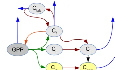
Figure 1. DALECv2 links the carbon pools (C) via allocation fluxes (green), litterfall fluxes (red) and decomposition (black). Respiration is represented by the blue arrows. The orange arrow represents the feedback of foliar carbon to gross primary produc-tion (GPP).

linear experiments. In Sect. 7 we discuss several extension to our manuscript and finally in Sect. 8 we draw conclusions.

2 Model, constraints and observations 2.1 DALECv2

Table 1.DALECv2 dynamical variables and parameters with their respective range. The units of the non-dimensionless quantities are given in brackets.

Label Variable Description Range

C₀(1) C_lab initial labile C pool (gC m−2) 20–2000

C0(2) Cf initial foliar C pool (gC m−2) 20–2000

C₀(3) Cr initial fine root C pool (gC m−2) 20–2000

C0(4) Cw initial above and below ground woody C pool (gC m−2) 100–105

C₀(5) Cl initial litter C pool (gC m−2) 20–2000

C0(6) Cs initial soil organic matter C pool (gC m−2) 100–2×105 p1 θmin litter mineralisation rate (day−1) 10−5–10−2 p2 fa autotrophic respiration fraction 0.3–0.7 p₃ f_f fraction of GPP allocated toC_f 0.01–0.5 p4 fr fraction of GPP allocated toCr 0.01–0.5 p5 clf annual leaf loss fraction (season) 1 - 8

p6 θw Cwturnover rate (day−1) 2.5×10−5–10−3 p7 θr Crturnover rate (day−1) 10−4–10−2 p8 θl Clturnover rate (day−1) 10−4–10−2 p9 θs Csturnover rate (day−1) 10−7–10−3 p10 2 temperature dependence exponent factor 0.018–0.08 p11 ceff canopy efficiency parameter 10 - 100

p12 donset leaf onset day (day) 1–365

p13 fl fraction of GPP allocated toClab 0.01–0.5 p14 cronset Clabrelease period (days) 10–100 p15 dfall leaf fall day (day) 1–365

p₁₆ c_rfall leaf fall period (days) 20–150

p17 clma leaf mass per area (gC m−2) 10–400

The meteorological drivers are extracted from 0.125◦_×0.125◦ _{ERA-Interim reanalysis data sets. For}

the purpose of our inverse modelling experiments we use four different observation streams: LAI, NEE, GPP and RESP (total respiration). LAI monthly mean observa-tions for AmeriFlux sites are extracted from MOD15A2 LAI 8-day version 005 1 km resolution product. These observations together with the meteorological drivers are provided by A. Bloom and J. Exbrayat. Details about their construction can be found in Bloom and Williams (2015). At AmeriFlux sites we use the level 4 data product (available at http://cdiac.ornl.gov/ftp/ameriflux/data/Level4/), which provides monthly means for NEE and GPP. NEE and GPP are then used to define RESP as RESP=NEE+GPP. The meteorological drivers span a period of 12 years from 2001 to 2013. LAI observations are available during the full period but for NEE and GPP, and thus RESP, shorter records are available depending on the AmeriFlux site. In this study we consider the Morgan Monroe State Forest located in Indiana, USA (39.3–86.4). This AmeriFlux site is composed in majority of mixed hardwood broadleaf deciduous trees and classifies as a humid subtropical climate.

In the remainder of the paper the main focus is on the vec-torx=log([p,C0])T: in Sect. 2.3 first where we investigate the sensitivity of different outputs with respect tox and its components, and then in subsequent sections wherexis

es-timated using inverse methods. The vectorx, denoting fixed quantities as initial conditions and parameters for the dynam-ical system DALECv2, is seen as the variable from the point of view of sensitivity analysis and inverse modelling and therefore its components will be referred to as state variables, input variables or parameters interchangeably throughout the manuscript.

2.2 Ecological constraints

Over the last decade many inverse modelling studies have used NEE measurements from the FLUXNET network, to-gether with other types of observations when available, to provide information about processes controlled by parame-ters with respect to which NEE is weakly sensitive. Though it contains an ever-increasing amount of information, the flux tower network only provides sparse coverage of terres-trial ecosystems. On the other hand, despite good spatial and temporal coverage, MODIS LAI monthly mean observations only constrain a limited set of DALECv2 state variables, and additional information is required in order to regularise the ill-posed problem and obtain a meaningful solution.

constraints, detailed in Bloom and Williams (2015), can be divided into two groups: static and dynamic constraints. The static constraints which directly impose conditions on the pa-rameters are as follows:

– Turnover rate constraints which ensure that turnover rates ratios are consistent with knowledge of the carbon pools residence times.

EDC1: p9< p8, (1)

EDC2: p9< p1, (2)

EDC3: p6<1/ (p5×365.25) , (3) EDC4: p7> p9expp10T , (4)

EDC5: p12+45< p15, (5)

where T denotes the mean temperature within the drivers time window. EDC4 is a modifica-tion to the constraint proposed in Bloom and Williams (2015). It is currently used in the CAR-DAMON framework (http://www.geos.ed.ac.uk/homes/ mwilliam/CARDAMOM.html).

– Root–foliar allocation which allows for a strong corre-lation between parameters controlling allocation to fo-liage and roots.

EDC6: froot<5(ffol+flab) , (6) EDC7: ffol+flab<5froot, (7) where the allocation fractionsffol,flabandfrootare de-fined as

fauto=p2, (8)

ffol=(1−fauto) p3, (9)

flab=(1−fauto−ffol) p13, (10) froot=(1−fauto−ffol−flab) p4. (11) The dynamic constraints, for which a model run is performed to define attractors, limit the application of the model to ecosystems with no major recent disturbance. They are de-fined as follows:

– Root–foliar mean dynamics

EDC8: Cr<5Cf, (12)

EDC9: Cf<5Cr, (13)

whereCfandCrdenote the mean ofCfandCrover the simulation period.

– Yearly carbon pools growth rate is limited to 10 %. EDC10−15: C

n

/C1<1+ζ (n−1)/10, (14) where for each poolCi denotes the mean carbon pool size over yeariand the growth factorζ is set to 1.

– Carbon pools are not expected to show rapid exponen-tial decay; therefore, parameter sets are required to sat-isfy the condition that the half-life period of carbon pools is more than 3 years.

EDC16−21: γ <3×365/log 2 (15) The trajectory of each carbon pool is approximated us-ing an exponential decay curvea+bexpγ t wherea, bandγ are the fitted exponential decay parameters and t the time variable, in days in this case.

– Carbon pools are expected to be within an order of mag-nitude of a steady-state attractor.

EDC22−29: C0/10< C∞<10C0, (16) where for each of the carbon poolsCs,Cl,CwandCr, C0denotes the initial state andC∞denotes the steady-state attractor defined as

C_som∞ =(fwood+(ffol+froot+flab) p1) G (p1+p9) p8expT p10

, (17)

C_lit∞=(ffol+froot+flab) G

p9expT p10 , (18)

C_wood∞ =fwoodG p6

, (19)

C_root∞ =frootG

p7 , (20)

whereG denotes the mean gross primary production andfwood,fsomandflitare given by

fwood=1−fauto−ffol−flab−froot, (21) f_som=f_wood+(froot+flab+ffol) p1/ (p1+p8) , (22)

flit=(froot+flab+ffol) . (23) To the original EDCs, we found it useful to add the three following constraints:

EDC30: LAI(summer) < α, α >0, (24)

EDC31: LAI(final day) >0, (25)

EDC32,33: −β < E[NEE]< β, β >0, (26) whereαandβ are real constants that need to be adjusted, LAI(summer) denotes the modelled LAI during summer and LAI(final day) denotes the modelled LAI at the end of the model run. These new constraints guarantee that LAI and the mean NEE remain within realistic bounds.

−0.1 0 0.1 0.2 0.3 0.4

mean MNS

NEE normalized sensitivity

p₂ p₅ p₁₇p₁₁p₁₃p₁₅C_s p₉ p₃ p₁₀C_f p₁₆C_L p₁₂p₄ p₈ p₁ C_w p₆ p₁₄p₇ C_r C_l

−0.1 0 0.1 0.2 0.3 0.4

mean MNS

LAI normalized sensitivity

p₁₇p₅ p₂ p₁₃p₁₁p₁₅p₃ C_f p₁₆C_L p₁₂p₁₄p₁ p₄ p₆ p₇ p₈ p₉ p₁₀C_r C_w C_l C_s

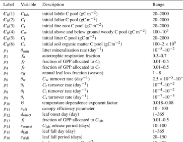
Figure 2. Mean normalised sensitivities (MNS): 100 parameter sets satisfying EDCs are sampled at the Morgan Monroe State Forest. Parameters are ranked in decreasing order according to their sensitivity, the blue dots represent the mean of the MNS (dimensionless quantity), the intervals represent 1σerror bars and the red dots correspond to null sensitivity.

2.3 Sensitivity analysis

Sensitivity analysis studies how the variations of the outputh

of a model can be attributed to variations of the input vari-ables xi. Such information is crucial for model design, in-verse modelling and reduction of complex non-linear mod-els. A global sensitivity analysis for DALEC was recently performed in Safta et al. (2015). Here we consider a local approach where first-order derivatives are used to build sen-sitivity indices that help us understand the influence of input variables on the output.

We denote ht as the function that maps x=log(p,C0) to the value of an output of the model (here LAI, NEE, GPP and RESP) at timet, and we denote the time series of the model output ash=(ht1, . . . , htN). Following Zhu and Zhuang (2014), we consider the mean normalised sensitiv-ity (MNS) defined as

si =E ∂h

∂xi |σi

σh

|X

j |∂h

∂xj σj

σh |

!

, (27)

where E(·) denotes the average of the time series. The scalarsσi andσhdenote the parameter variance, set as 40 % of the parameter range, and the variance of the output respec-tively. The partial derivatives are computed using the adjoint derived using the method described in Giering and Kaminski (1998). The MNSsi is a dimensionless number that allows us to compare among parameters.

We consider the Morgan Monroe State Forest over a 12-year period. We sample 100 parameter sets satisfying the ecological constraints. For each parameter set, we compute the MNS for DALEC simulated mean fluxes LAI and NEE. In Fig. 2 parameters are ranked with respect to their mean

MNS. We see that for LAI only 12 out of the 23 variables are sensitive, namelyp5,p17,p2,p13, p11,p15, p16,Cf,p12, p3, Clab andp14. Therefore, using LAI only in an inverse modelling experiment provides, at best, information about those twelve sensitive variables. For NEE we see that all vari-ables are sensitive. Sensitivity analysis for GPP shows simi-lar characteristics with LAI and so does RESP with NEE. For the four outputs under consideration (LAI, NEE, GPP and RESP) the most sensitive variables are the autotrophic respi-ration,p2, the annual leaf loss fraction,p5, the leaf mass per area,p17, the fraction of GPP allocated to labile pool,p13, the nitrogen use efficiency,p11, and the leaf fall dayp15.

Here our focus is on the mean of the time series of DALEC fluxes (LAI, NEE) over a 12-year period. Finer analysis could be carried out by looking at seasonal aspects of the carbon cycle, identifying what variables are the most sensi-tive at certain times of the year, for example as studied in Safta et al. (2015).

3 Data assimilation

In this section we introduce concepts and methods that al-low for close mathematical scrutiny of inverse problems and we present the variational method that we will apply in the following sections.

3.1 Ill-posed problem

A generic inverse problem consists of finding an dimen-sional state vectorxsuch that

for a given N-dimensional observation vector y, including random noise, and a given modelh. In the remainder of the paper the terms state vector, state variable, input variable and parameters will be used interchangeably to denote the vec-torxto be estimated using inverse methods and defined in the previous section asx=log([p,C])T. The problem is well posed in the sense of Hadamard (1923) if the three following conditions hold: (1) there exists a solution, (2) the solution is unique and (3) the solution depends continuously on the input data. If at least one of these conditions is violated the problem is said to be ill-posed. The inverse problem (Eq. 28) is often ill-posed, and a regularisation method is required to replace the original problem with a well-posed problem. Solving Eq. (28) amounts to (1) constructing a solution x, (2) assessing the validity of the solution and (3) characteris-ing its uncertainty. Each inverse problem has its own features which need to be understood in order to characterise properly the solution and its uncertainty.

3.2 Bayesian inference: 4DVAR

Inverse problems are generally presented in a probabilistic framework where most methods can be expressed through a Bayesian formulation. The Bayesian approach provides a full characterisation of all possible solutions, their relative probabilities and uncertainties.

From Bayes’ theorem, the probability density func-tion (PDF) of the model state x given the set of observa-tionsy,p(x|y), is given by

p(x|y)∝p(y|x)p(x), (29)

where p(y|x)is the PDF of the observations given x and p(x)is the prior PDF of x. A special case is given when p(y|x)andp(x)are Gaussian PDF given by

p(x)=exp

−1

2(x−x0)

T_B−1_(x−x0)

, (30)

and

p(y|x)=exp

−1

2(h(x)−y)

T_R−1_(h(x)−y)

, (31)

whereBis the covariance matrix of the prior termx0, and Ris the covariance matrix of the observation error. When the operatorhis linear then the posterior PDFp(x|y)is Gaus-sian and thus fully characterised by its mean and covariance matrix. The mean is obtained by minimising the modulus of the log of the joint probability distribution, which is the cost functionJ given by

J (x)=J₀(x)+Jy(x)=

1

2kx−x0k

2

B+

1

2kh(x)−yk

2

R. (32)

Many methods can be considered to minimise this cost func-tion. A Monte Carlo method is employed in Bloom and Williams (2015). Here we use a variational approach which

applies a gradient-based method where the gradient is given by

∇J=B−1(x−x0)+HTR−1(h(x)−y), (33) withHT denoting the adjoint operator. The covariance matrix of the solution,C, is given by the inverse of the Hessian of the cost function

C= [Hess(J )]−1=hB−1+HTR−1Hi

−1

. (34)

When the observation operatorhis non-linear, the cost func-tionJ can have multiple local minima and the posterior PDF may no longer be a Gaussian PDF. However, locally, the PDFN (_ex,C), whereCis given by Eq. (34) evaluated at a minimum_ex, provides a Gaussian approximation of the pos-terior PDFp(x|y).

The first term in the cost function (Eq. 32) is a regularisa-tion term encoding the Gaussian priorp(x). As we will show in the next sections the problem of assimilating Earth ob-servations (LAI, GPP, NEE, RESP) into DALEC is a highly ill-posed problem and regularisation is required. The sensi-tivity analysis of Sect. 2.3 showed that LAI and GPP are not sensitive to all variables. Moreover, all observations streams show very low sensitivities to some variables. Therefore, as will be illustrated in Sect. 4.1, the solution (if any) is likely to be subject to large uncertainties. Apart from a couple of extensively studied sites, our prior knowledge about the vari-ables is so far limited to their upper and lower bounds given in Table 1. As performed in Zhu and Zhuang (2014), it is a common practice to use this information to define a Gaus-sian priorp(x)∼N (x0,B), wherex0is given by the centre of the variables ranges andBis the diagonal matrix whose diagonal elements are the squares of 40 % of the variables ranges. While using this kind of regularisation is necessary to ensure any solution at all when no better source of informa-tion is available, this introduces some biases in the soluinforma-tion. The EDCs introduced by Bloom and Williams (2015) pro-vide new prior information about the variables. One of the purposes of this paper is to incorporate the EDCs as a regu-larisation term within 4DVAR. In the next section we propose a strategy to achieve this goal.

3.3 EDCs and 4DVAR

Incorporating the EDCs from an optimisation point of view can be easily performed by considering an inequality con-straint optimisation problem where we aim at solving minxJy(x)subject tol<x<uandg(x) <0,

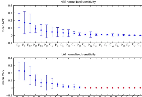
We are seeking a multivariate Gaussian distribution that would encode the EDCs. At a forest site, we start by sam-pling the parameter space to obtain an ensemble of 1000 pa-rameter sets satisfying the EDCs; each papa-rameter set x is randomly created and required to satisfy g(x) <0. We de-note this ensemble byXEDCs. For most parameters, the sam-pling gives rise to undetermined PDFs which can certainly not be represented by Gaussian PDFs. However, upon in-specting the distribution g(x), for all x inXEDCs, we see that the distribution log(g(x)) can be fairly accurately ap-proximated by multivariate Gaussian PDFsN (c,6), where

cdenotes the mean of the distribution log(g(x))and6 de-notes its covariance matrix. As an example, Fig. 3 shows the marginals log(g4(x)) and log(g6(x)), corresponding to the EDCs 4 and 6 respectively, together with a Gaussian fit.

Using Bayes’ theorem we can then write

p(x|y,c)∝p(y|x)p(c|x)p(x). (35) Finding a Gaussian approximation for p(x|y, c) amounts then to minimising the cost function

J (x)=1

2kh(x)−yk 2 R+

1

2klog(g(x))−ck 2 6

+1

2kx−x0k 2

B. (36)

The gradient ofJ is given by

∇J (x)=HTR−1(h(x)−y)+ 1

g(x)G

T₆−1_{(log(g(x))−c)}

+B−1(x−x0) ,

and the Hessian of the cost function can be approximated by

2=HTR−1H− 1

(g(x))2GG

T₆−1_{(log(g(x))−c)}

+ 1

(g(x))2G

T₆−1_G+B−1_{, (37)}

evaluated at the minimiser_ex. The operatorGT _{denotes the} adjoint of the tangent linear modelGwhose key ingredient is given by the adjoint of DALECv2. The approximation of p(x|y,c) is then given by the Gaussian distribution N (_ex,

2−1). In Sect. 5 we will perform experiments using real data to validate this approach.

4 Linear analysis

Considerable theoretical insights into the nature of the in-verse problem, and the ill-posedness, can be obtained by studying a linearisation of the operator h. A first approxi-mation to the inverse problem consists of finding a perturba-tionzwhich best satisfies the linear equation

Hz=d, (38)

−150 −10 −5 0 0.1

0.2 0.3 0.4

EDC₄

Density

log(|g₄(x)|) −6 −4 −2 0 2 0

0.2 0.4 0.6 0.8

EDC₆

Density

log(|g₆(x)|)

Figure 3.Distribution and Gaussian fit for EDC4and EDC6.

whereHis the tangent linear operator forhandd is a per-turbation of the observations. The linear operatorHis com-monly referred to as theobservability matrix (see Johnson et al., 2005). The least squares formulation of this problem is to solve the optimisation problem

minzJ (z)=minz 1

2kHz−dk

2_{. (39)}

The minimisation can be performed using an iterative method such as the conjugate gradient method, where the gradient is given by

∇J=HT(Hz−d). (40)

The inverse Hessian of the cost function,(HTH)−1, gives the covariance matrix of the least squares solution. In the next section we consider a direct solution method based on the singular value decomposition of the operatorH, which al-lows us to investigate the nature of the ill-posedness of the problem. We illustrate regularisation using a truncated sin-gular value decomposition.

4.1 Singular value decomposition

We consider a singular value decomposition ofHof the form

H=USVT, (41)

whereUis aN×Nunitary matrix,Vis an×nunitary ma-trix andSis theN×ndiagonal matrix whose diagonal el-ements are the singular valuess1≥. . .≥sn≥0. Using this decomposition, the solutionzLSto Eq. (39) can be written as

zLS=VS†UTy=H†y. (42)

The matrixH†=V S†UT is thepseudo-inverseofHwhere S†is the diagonal matrix obtained by transposingSand re-placing the non-zero elements with their inverses_i−1. The covariance of the solution is given by

Cov(zLS)=H†TH†. (43)

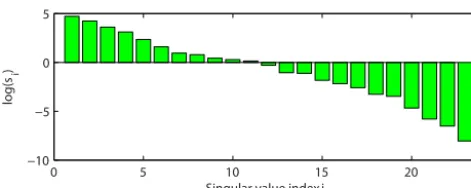
0 5 10 15 20 −10

−5 0 5

Singular value index i

log(

si

)

Figure 4.Singular values of the observability matrix for NEE (log scale).

1996) that the relative error in the solution, defined as the left-hand side of the above inequality, is bounded by

kzLS−z0k kz0k

≤κ(H)kk

kdk, (44)

where κ(H) is the condition number of H defined as κ(H)=s1/sn,z0 denotes the truth (possibly unknown) and

represents observational noise. When the condition number is large the matrix is said to be ill-conditioned, the problem is ill-posed and the solution (Eq. 42) is unstable: small per-turbations to the system can lead to very large perper-turbations in the solution.

4.2 Stability for NEE operator

As an example we consider the problem of assimilating NEE observations into DALECv2 to estimate model parameters and initial conditions at Morgan Monroe State Forest. We linearise Eq. (28) about a pointx∗_{satisfying the EDCs, form}

the observability matrix H and compute its singular value decomposition. The singular values, shown in Fig. 4, reveal a condition number of the order of 105.

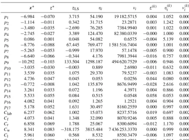
For a signal-to-noise ratio, namely kk/kdk, of magni-tude 0.1, inequality (Eq. 44) gives an upper bound for the relative error in the solution of the order of 104, which does not give much credit to the least squares solution. How sharp is this bound? Are we overestimating the error? To answer these questions we create a set of noisy observations with noise varianceσ=0.1 and we compute the solution (Eq. 42). The relative error for each component of the solution,ηi, and the varianceνi, are given in Table 2. Despite a relatively good match between the modelled NEE perturbations and the ob-servations, as shown in Fig. 5, the results of Table 2 show very large relative errors and variances for most variables. Moreover, these results are in agreement with the results of REFLEX: parameters directly linked to foliage and GPP are better estimated than parameters related to allocation to and turnover of fine root/wood. The results of Table 2 reflect the sensitivity analysis shown in Fig. 2. The variables with re-spect to which NEE is the most (least) sensitive are the less (more) affected by the noise.

To reduce the impact of observational noise on the solu-tion, regularisation is required. The truncated singular value

2001 2002 2003 2004 2005

−2 −1 0 1 2

Year

NEE (gCm

−2

day

−1)

Figure 5.Solution of the linearised inverse problem for NEE. The red points represent the observations, the red curve is the true tra-jectory, the green curve is the trajectory obtained using the unstable solution and the blue curve is obtained using the truncated singular value decomposition (TSVD) solution.

decomposition (TSVD) is a simple and popular method for regularisation. TSVD consists of truncating the pseudo-inverse in Eq. (42) in order to remove the smallest singular values, the most affected by the noise. The solutionz(k) _is then given by

z(k)=VkS†_kUTky=H

†

ky, (45)

wherekis the truncation rank and whereSk,UkandVk are the rectangular matrices formed by the firstkcolumns ofS, UandV. The covariance of the solution is given by

Covz(k)=Vk

S†_k

−2

VT_k. (46)

The truncation rank k can be chosen using the L-curve method. The L curve is a log–log plot of the norm of the solutionkz(k)kagainst the norm of the residualkHz(k)−dk parametrised by the regularisation parameterk. The optimal parameter corresponds to the point of maximum curvature of the L curve. Further details on the L-curve method can be found in Hansen and O’Leary (1993).

Table 2.Results of the linear inverse problem showing (1) the solution components for the least squares solutionz_LS together with their relative errorηi (dimensionless quantity) and varianceνi and (2) the solution components for the TSVD solutionz(k)together with their relative errorη(k)_i and varianceν_i(k).

x∗ z∗ zLS ηi νi z(k) η(k)_i ν(k)_i

p1 −6.984 −0.070 3.715 54.190 19 182.5715 0.004 1.052 0.0001 p2 −1.114 −0.011 0.342 31.715 23.2871 0.003 1.242 0.0005 p3 −3.480 −0.035 −2.690 76.285 7384.9940 0.001 1.022 0.0000 p4 −2.745 −0.027 3.389 124.470 82 380.0339 −0.000 1.000 0.0000 p5 0.086 0.001 0.048 54.082 0.6575 −0.004 5.139 0.0009 p6 −8.776 −0.088 67.445 769.477 1 581 516.7404 0.000 1.001 0.0000 p7 −5.265 −0.053 −0.999 17.970 57.1478 −0.005 0.900 0.0001 p8 −6.640 −0.066 −0.344 4.176 7981.3944 −0.016 0.757 0.0013 p9 −10.292 −0.103 133.504 1298.187 494 620.7529 −0.006 0.946 0.0002 p10 −3.035 −0.030 −0.003 0.889 2.6980 −0.011 0.632 0.0008 p11 3.539 0.035 1.075 29.370 79.5237 −0.003 1.083 0.0003 p12 4.736 0.047 0.045 0.053 0.0256 0.044 0.080 0.0003 p13 −0.772 −0.008 1.042 135.879 8676.9499 −0.028 2.616 0.0033 p14 3.261 0.033 0.072 1.196 4.3971 0.004 0.866 0.0001 p₁₅ 5.533 0.055 0.084 0.515 0.0548 0.058 0.053 0.0003 p16 4.082 0.041 0.092 1.265 1.2521 0.004 0.904 0.0001 p17 5.178 0.052 1.631 30.497 8160.2559 0.000 0.997 0.0005 Clab 6.237 0.062 1.002 15.073 8237.5716 0.019 0.697 0.0020 Cf 4.073 0.041 1.348 32.090 8070.9246 0.005 0.888 0.0001 Cr 6.858 0.069 1.788 25.067 8300.6094 −0.012 1.170 0.0008 Cw 8.341 0.083 −318.175 3815.484 7 436 253.3370 0.000 0.999 0.0000 Cl 5.961 0.060 0.568 8.532 8550.3479 −0.006 1.097 0.0002 Cs 8.956 0.090 −134.334 1500.869 483 025.4281 −0.006 1.064 0.0002

4.3 Resolution matrix

As suggested by Eqs. (42) and (45), finding a solution z

amounts to constructing ageneralised inverseHg such that formally

z=Hgd. (47)

The generalised inverse is the operator representing any method, direct or iterative, used to solve the linear inverse problem, with or without any kind of regularisation. In the previous section we considered two examples of generalised inverse, the pseudo-inverse and the truncated inverse ob-tained using TSVD. The generalised inverse can be used to define operators which directly address the conditions for well-posedness for the linearised problem. Assuming a true state z∗ exists, possibly unknown, using Eqs. (38) and (47) we can then define an operatorNcalled themodel resolution matrixwhich relates the solutionzto the true state

z=HgHz∗=Nz∗. (48)

This matrix provides a practical tool to analyse the resolution power of an inverse method, that is, its ability to retrieve the true state, with or without using any regularisation method: the closerNis to the identity, the better the resolution. More-over, the trace of the matrix defines a natural notion of infor-mation content (IC). Similarly adata resolution matrixcan

be defined to study how well data can be reconstructed and its diagonal elements naturally define a notion ofdata impor-tance. For the two examples of generalised inverse presented in the previous section we obtain the following resolution matrices:

N=H†H, (49)

for the pseudo-inverse and

N=VkVTk, (50)

for the truncated pseudo-inverse. In the first case the IC equals the number of non-zero singular values, in the sec-ond case the IC equals the truncation rankk. An in-depth theoretical and practical analysis of these concepts and those introduced in the remainder of this section can be found in Menke (1984).

While the model resolution matrix allows us to see how a solution strategy maps the true state variables to the solution of the inverse problem, and to see how well and how indepen-dently the state variables can be recovered, one also needs to assess the uncertainty of the solution. This can be studied us-ing the so-calledunit covariance matrix,C, defined using the generalised inverse as

p1 p2 p3 p4 p5 p6 p7 p8 p9 p10 p11 p12 p13 p14 p15 p16 p17 Cla Cf Cr Cw Cl Cs p1

p2 p3 p4 p5 p6 p7 p8 p9 p10 p11 p12 p13 p14 p15 p16 p17 Cla Cf Cr Cw Cl

Cs −0.2

0 0.2 0.4 0.6 0.8 1

Figure 6.Model resolution matrix for the LAI operator.

By characterising the degree of error amplification that oc-curs in the mapping from the true state to the solution of the inverse problem, the unit covariance matrix is a crucial object for studying the stability of the solution with respect to observational noise. The unit covariance matrix defined by Eq. (51) agrees with the covariance matrices given in the previous section by Eq. (43) for the pseudo-inverse, and by Eq. (46) when TSVD is applied.

4.4 Resolution for LAI operator

We now study the model resolution matrix for the LAI ob-servation operator at Morgan Monroe State Forest. In the first instance we will demonstrate the resolution power of the LAI signal without regularisation using the pseudo-inverse as generalised inverse first, and then apply TSVD to show how using the truncated pseudo-inverse affects resolution. In a second case we will study the added value of the EDCs in terms of resolution.

As previously, we linearise Eq. (28) about the point x∗

given in Table 2. The trace of the resolution matrix obtained using the pseudo-inverse as generalised inverse is 10, and this means that 10 independent variables can be estimated using LAI. These independent variables are not the variables in which the system is expressed, but a linear transformation can be found to express the system in terms of the indepen-dent variables. Figure 6 shows the model resolution matrix for LAI. As shown in Sect. 2.3 with the sensitivity analysis, 11 out of the 23 variables are not sensitive to LAI, and this can be seen in the resolution matrix by the diagonal terms which are zero, represented in blue. In contrast the diagonal elements corresponding to sensitive variables have positive values, represented by colours ranging from light blue to red. Figure 6 also shows that whereasp5,p11,p12,p14,p15and p16 are perfectly resolved (the corresponding elements are coloured brown or dark red), there exist linear combinations between the remaining sensitive variables, which explains

−10 −5 0 5 10

p₂ p₃ p₅ p₁₁ p₁₂ p₁₃ p₁₄ p₁₅ p₁₆ p₁₇ C_lab C_f

log variances

Figure 7.Diagonal elements (log scale) of the unit covariance ma-trix for the LAI operator: using the pseudo-inverse shown in green and TSVD shown in yellow.

why only 10 independent variables can be estimated from the 12 sensitive variables.

For the study of the unit covariance matrix we restrict our-selves to the sensitive variables. This amounts to removing the columns corresponding to the non-sensitive variables, containing only null elements, from the observability ma-trix. The dependency of the solution on observational noise can be studied by looking at Fig. 7, where the diagonal el-ements of the unit covariance matrix, corresponding to the variance of each element of the solution obtained using the pseudo-inverse, are represented in log scale. Except forp5, p12,p15andp16, all variances are shown to be large.

As previously, we illustrate a simple regularisation strat-egy, TSVD, and show its effects on both resolution and sta-bility. Figure 8 shows the resolution matrix for LAI with op-timal truncation rankk=6. The IC decreases to 6. We see that whereasp5,p12,p15 andp16 remain almost perfectly resolved,p13,p17 andClab are only partially resolved and the remaining variables are not resolved properly. Figure 7 shows the corresponding diagonal elements of the unit co-variance matrix, from which we see that the co-variances have been drastically reduced. This example shows how regulari-sation ensures stability at the price of losing resolution.

We now consider the effect of incorporating the static EDCs into the variational framework in terms of resolution. The static EDCs are given by the first seven EDCs, the linear problem is then given by

_H

e

G

z=

d f

, (52)

where

e

G=g x∗−16−1/2G, (53)

p2 p3 p5 _{p11 p12 p13 p14 p15 p16 p17 Cl}a Cf

p2 p3 p5 p11 p12 p13 p14 p15 p16 p17 Cla Cf

−0.2 0 0.2 0.4 0.6 0.8

Figure 8.Model resolution matrix for the LAI operator using TSVD with truncation rankk=5.

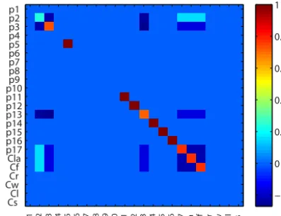
p1 p2 p3 p4 p5 p6 p7 p8 p9 p10 p11 p12 p13 p14 p15 p16 p17 Cla Cf Cr Cw Cl Cs p1

p2 p3 p4 p5 p6 p7 p8 p9 p10 p11 p12 p13 p14 p15 p16 p17 Cla Cf Cr Cw Cl Cs

−0.2 0 0.2 0.4 0.6 0.8 1

Figure 9.Model resolution matrix for LAI and static EDCs as de-fined by Eq. (52).

model resolution matrix corresponding to the operator on the left-hand side of Eq. (52), obtained using the pseudo-inverse, is depicted in Fig. 9. The trace of the model resolution ma-trix gives an IC of 16, 13 variables are perfectly resolved and 4 variables show linear dependencies (p2,p3,p4andp13). However, although p9 andp10 are sensitive variables, they do not appear to be resolved at all: inspecting the linear op-eratorGshows that the non-zero components corresponding top9andp10are several order of magnitude smaller than the other components.

This example shows clearly the benefit of introducing the static EDCs to help estimate poorly constrained or otherwise undetermined components.

5 Experiments at AmeriFlux sites

We now consider a real experiment at the Morgan Monroe State Forest. At this AmeriFlux site, 12 years of MODIS LAI monthly mean observations from 2001 to 2013, NEE, GPP

Table 3.Experiment set up summary: in Exp. 1 we use LAI and bounds constraints (BDS), in Exp. 2 we use LAI, NEE and BDS and so on.

LAI NEE GPP RESP BDS EDCs

Exp. 1 x x

Exp. 2 x x x

Exp. 3 x x x x x

Exp. 4 x x x

Exp. 5 x x x x

Exp. 6 x x x x x x

and thus RESP observations from 2001 to 2005 are avail-able. Our goal is to study two different aspects. The first one is the impact of using multiple data streams: how does it af-fect uncertainty of the predicted fluxes and how well do we predict non-observed fluxes? The second one is to use the static EDCs and to assess their utility in constraining poorly sensitive variables.

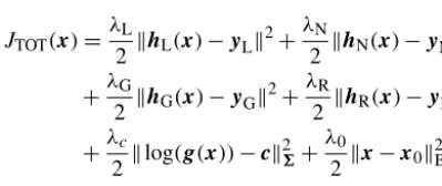
When including all terms the cost function,JTOT, becomes JTOT(x)=

λL

2 khL(x)−yLk 2₊λN

2 khN(x)−yNk 2

+λG

2 khG(x)−yGk 2₊λR

2 khR(x)−yRk 2

+λc

2 klog(g(x))−ck 2

6+

λ0

2 kx−x0k 2 B =JL+JN+JG+JR+Jc+J0,

where subscripts L, N, G and R stand for LAI, NEE, GPP and RESP respectively. The vectorsy_L,y_N,y_Gandy_Rrepresent the observation vectors for LAI, NEE, GPP and RESP re-spectively. The scalarsλL,λN,λG andλRtake the value 0 or 1 depending on whether or not the corresponding data stream is included in the experiment. The scalarλctakes the value 0 or 1 depending on whether we include the EDCs and λ0takes the value 1.

We perform six experiments summarised in Table 3. In ex-periment (Exp.) 1, we use only LAI observations and bounds constraints so that in the cost functionJTOT we set λL=1 andλ0=1, and the otherλs are set to zero. For Exp. 2, we use LAI and NEE observations, that is, we setλL=1,λN=1 andλ0=1; the otherλs are set to zero. We proceed simi-larly for the remaining experiments. Here we assimilate all data streams simultaneously; it is not our intention to ques-tion what method best accommodates multiple data streams. MacBean et al. (2016) addresses this question using a simple C cycle model. Moreover, we choose to assume the same sta-tistical error for all data streams and set their error covariance matrix equal to the identity. To avoid being trapped at mean-ingless local minima, the experiments are performed multiple times using different initialisation parameter sets and results for the best candidate only are reported.

2001 2002 2003 2004 2005 2006 2007 2008 2009 2010 2011 2012 2013 0

2 4 6

Year

LAI

2001 2002 2003 2004 2005 2006 2007 2008 2009 2010 2011 2012 2013 −8

−6 −4 −2 0 2

Year

NEE (gCm

−2

day

−1)

Figure 10.DALECv2 monthly estimates for LAI and NEE at Mor-gan Monroe State Forest. The red dots are the observations, the blue trajectories are obtained using the 4DVAR analysis, and the grey tra-jectories are ensemble runs obtained from a 95 % confidence sample of the posterior PDF.

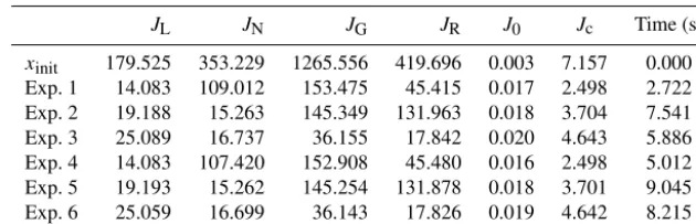
in Table 5, where the solution components and their vari-ance are presented for all experiments. Results of Table 4 show that JL is the smallest in Exp. 1 when LAI only is used. In Exp. 2, when adding NEE we see thatJNdecreases from 109.012 in Exp. 1 to 15.263, andJGslightly decreases as compared to Exp. 1, but JRincreases instead. In Exp. 3 we see that all costs drastically decrease compared to their initial values. Going from Exp. 1 to Exp. 3, J0slightly in-creases; adding more data streams constrains more param-eters, and the parameters shift from their prior value which may causeJ0to increase. Similar observations can be made for Exp. 4 to Exp. 6; moreover, we see that including the EDCs only slightly affects the costs. A reason for this might be that EDCs help constrain the less sensitive parameters for which the costs are less sensitive, as suggested by the sen-sitivity analysis depicted in Fig. 2. To see the effect of the EDCs we need to look at Table 5, which details the solution components together with their relative variance defined by the ratio of the variance by the parameter range. In Exp. 1 we see that the variables with the smallest relative variance are the most sensitive parameters as illustrated in Fig. 2:p2,p5, p10,p12,p14,p15,p16andp17. We recall that the sensitivity analysis of Sect. 2.3 was performed by averaging sensitivi-ties for an ensemble of initial parameter sets; therefore, the ranking shown in Fig. 2 may not be reflected in the relative variances. As we include NEE in Exp. 2 we see that most relative variances decrease, especially forp8,p9,p10,p13, Clab, Cf andCl. The only variable whose relative variance increases is p14, but as shown in Fig. 2, p14 has very low sensitivity. In Exp. 3 most relative variances decrease. The values are still large though forp1,p3,p4,p6,p9,CrandCl. Again, similar features can be observed for Exp. 4 to Exp. 6,

2001 2002 2003 2004 2005 2006 2007 2008 2009 2010 2011 2012 2013 0

5 10 15

Year

GPP (gCm

−2

day

−1)

2001 2002 2003 2004 2005 2006 2007 2008 2009 2010 2011 2012 2013 0

2 4 6 8

Year

RESP (gCm

−2

day

−1)

Figure 11.DALECv2 monthly estimates for GPP and RESP at Morgan Monroe State Forest. The red dots are the observations, the blue trajectories are obtained using the 4DVAR analysis, the grey trajectories are ensemble runs obtained from a 95 % confidence sample of the posterior PDF.

but a clear improvement can be seen for most variables ex-cept forCrwhich is not constrained by the first seven EDCs. Finally, the last column of Table 4 shows the computation time for each experiment. As expected we see that the more observation streams we consider, the longer the experiment takes to run, and incorporating the EDCs increases compu-tation time. However, we stress that these figures are several orders of magnitude less than the time required to perform the same experiments using the current gold standard MCMC approach used in Bloom and Williams (2015).

Figures 10 and 11 show the predicted fluxes for LAI, NEE, GPP and RESP for the result of Exp. 6. We can see good agreement between modelled fluxes and observations. The uncertainty of the predicted fluxes is evaluated by modelling an ensemble of trajectories from a 95 % ellipsoid of the pos-terior truncated Gaussian distribution. These trajectories are represented as grey curves in Figs. 10 and 11. Figure 12 shows the posterior parameter distribution marginals forp1, p7,p16andCffor Exp. 6, illustrating the four different cases where most of the marginal is contained in the parameter range forp16; the marginal is truncated on the left or the right forp7andCfand truncated on both sides forp1.

6 DALEC-SP

Table 4.Costs for the results of the inverse modelling experiments. The last column reports the computation time in seconds for the experi-ment.

JL JN JG JR J0 Jc Time (s)

xinit 179.525 353.229 1265.556 419.696 0.003 7.157 0.000 Exp. 1 14.083 109.012 153.475 45.415 0.017 2.498 2.722 Exp. 2 19.188 15.263 145.349 131.963 0.018 3.704 7.541 Exp. 3 25.089 16.737 36.155 17.842 0.020 4.643 5.886 Exp. 4 14.083 107.420 152.908 45.480 0.016 2.498 5.012 Exp. 5 19.193 15.262 145.254 131.878 0.018 3.701 9.045 Exp. 6 25.059 16.699 36.143 17.826 0.019 4.642 8.215

−10 −8 −6

0 0.05 0.1 0.15 0.2

p₁ range

Density

3.5 4 4.5

0 1 2 3 4

p₁₆ range

Density

−9 −8 −7 −6 −5

0 0.1 0.2 0.3 0.4

p₇ range

Density

3 4 5 6 7

0 0.5 1

C_f range

Density

Figure 12.Posterior parameter distributions for parametersp1,p7, p16andCffor Exp. 6. For each plot the limits of the abscissa cor-respond to the parameter range. The red curve is the Gaussian pos-terior distribution and the blue bars represent the sample used to produce the grey trajectories in Figs. 10 and 11.

As shown in Chuter et al. (2015) for the previous DALEC evergreen and deciduous models, the evolution of the carbon pools for DALECv2 show a tipping point which depends on the parametersp1 top17. Given a set of parameters,p, the fast carbon poolsClab,Cf,CrandCl grow or decay rapidly to an equilibrium state. This equilibrium is either zero and the forest dies out or a pseudo-periodical seasonal cycle as shown in Fig. 13 forCf. Moreover, there exists a limit value below which any initial condition leads to the zero equilib-rium and above which the equilibequilib-rium is a strictly positive pseudo-periodical seasonal cycle.

Here we consider ecosystems with no recent major distur-bance, where the fast carbon pools are expected to be close to their pseudo-periodical cycle. To model these ecosystems, one can either restrict the parameter space by using the dy-namic EDCs, or we can introduce a spin-up period during which the carbon pools reach their attractor. Given param-eters p1 top17 and initial values forCw andCs a first run of DALECv2 is performed to obtain a state which is closer

to a pseudo-periodical cycle for the fast carbon pools. The steady-state trajectories are then used to initialise the fast car-bon pools. For this DALECv2 “spin-up” model, DALEC-SP, the state variable is therefore formed of the 17 parameters, p1, . . . ,p17, and the initial conditions forCwandCs.

DALEC-SP offers several advantages: some of the EDCs such as those controlling the growth and the half-life pe-riod of carbon pools are almost automatically satisfied. This greatly reduces the time required to generate the PDFp(c|x). Moreover, as the sensitivity analysis and the resolution ma-trices showed, the fast carbon pools are variables that are not highly sensitive to the signals that we observe, and therefore reducing the number of variables by removing the fast car-bon pools is likely to improve the overall conditioning of the inverse problem. Reproducing experiments 1 to 6 using DALEC-SP shows similar results to those with DALECv2.

7 Discussion

optimisa-Table 5.Results of the inverse modelling experiments. The solution components together with their relative variance, in brackets, are given for each experiment. The vectorxinitis the randomly chosen parameter set satisfying the EDCs that initialises the minimisation routine.

xinit Exp. 1 Exp. 2 Exp. 3 Exp. 4 Exp. 5 Exp. 6

p₁ −5.172 −8.059 (1.727) −8.248 (1.471) −8.282 (1.021) −5.954 (0.112) −5.901 (0.075) −6.499 (0.057) p₂ −0.947 −0.885 (0.207) −1.106 (0.120) −1.085 (0.030) −0.848 (0.171) −0.982 (0.138) −0.984 (0.020) p₃ −4.318 −2.673 (0.955) −2.944 (0.849) −3.376 (0.894) −3.073 (0.954) −4.603 (0.973) −3.510 (0.895) p₄ −1.493 −2.649 (0.978) −2.813 (0.961) −2.692 (0.936) −1.589 (0.155) −1.386 (0.091) −1.476 (0.095) p₅ 1.123 0.117 (0.003) 0.153 (0.002) 0.085 (0.000) 0.135 (0.002) 0.010 (0.000) 0.090 (0.000) p₆ −7.959 −8.752 (0.922) −8.870 (0.911) −8.707 (0.919) −6.910 (0.144) −7.933 (0.886) −8.330 (0.883) p₇ −7.432 −6.908 (1.151) −6.373 (0.941) −5.064 (0.224) −7.336 (0.225) −7.015 (0.207) −6.241 (0.320) p₈ −5.281 −6.908 (1.151) −6.906 (0.316) −6.522 (0.078) −5.768 (0.107) −4.981 (0.049) −6.144 (0.034) p₉ −16.012 −11.513 (2.303) −10.075 (0.995) −11.411 (1.514) −10.563 (1.141) −15.973 (2.298) −11.043 (0.848) p₁₀ −3.041 −3.272 (0.373) −3.296 (0.085) −3.036 (0.055) −3.255 (0.371) −2.689 (0.077) −3.037 (0.051) p₁₁ 2.792 3.829 (0.540) 4.026 (0.163) 3.542 (0.003) 3.958 (0.458) 3.573 (0.120) 3.548 (0.003) p₁₂ 3.549 4.626 (0.002) 4.739 (0.000) 4.735 (0.000) 4.625 (0.002) 4.663 (0.001) 4.736 (0.000) p13 −1.768 −0.693 (0.130) −0.996 (0.067) −0.795 (0.046) −0.930 (0.077) −0.761 (0.026) −0.813 (0.033) p₁₄ 3.343 4.013 (0.034) 3.291 (0.123) 3.292 (0.052) 3.968 (0.030) 3.762 (0.009) 3.248 (0.077) p₁₅ 5.656 5.512 (0.001) 5.528 (0.001) 5.531 (0.000) 5.518 (0.001) 5.626 (0.000) 5.533 (0.000) p₁₆ 4.529 4.115 (0.068) 3.993 (0.025) 4.095 (0.011) 4.050 (0.063) 4.463 (0.009) 4.100 (0.010) p₁₇ 5.351 5.289 (0.213) 5.278 (0.198) 5.138 (0.165) 5.129 (0.180) 5.051 (0.104) 5.082 (0.106) C_lab 3.979 5.950 (0.115) 6.031 (0.059) 6.187 (0.040) 5.792 (0.103) 5.026 (0.143) 6.106 (0.027) C_f 5.389 4.677 (0.282) 4.868 (0.068) 4.038 (0.066) 4.542 (0.263) 5.806 (0.062) 4.152 (0.043) Cw 7.045 5.298 (1.151) 5.829 (0.900) 6.520 (0.096) 5.329 (1.149) 7.165 (0.265) 7.093 (0.232) Cr 9.753 8.406 (1.554) 8.188 (1.533) 8.318 (1.544) 8.453 (1.541) 9.612 (1.553) 8.114 (1.531) C_l 3.992 5.298 (1.151) 7.307 (0.300) 6.226 (0.161) 5.354 (1.141) 4.534 (0.438) 6.015 (0.089) Cs 9.721 8.406 (1.900) 9.546 (1.188) 8.603 (1.633) 8.889 (1.528) 9.615 (1.899) 8.448 (1.559)

2001 2002 2003 2004 2005 2006 2007 2008 2009 2010 2011 2012 2013 0

500 1000 1500

Cf

(gCm

−2day −1)

Year

Figure 13.Pseudo-periodical seasonal cycle for DALECv2. Using a given set of parameters and initial values forCwandCs, 100 DALECv2 runs are performed using random initial values forClab,Cf,Cr,Cl. The plot shows the 100 trajectories forCf.

tion as stated in Sect. 3.3 and adding a penalty term to ac-count for the EDCs. The latter solution which is the main interest of this publication was found to be the most success-ful in our case.

The complexity of global-scale experiments still limit the application of fully non-linear methods such as MCMC. In Ziehn et al. (2012) a comparison between the MCMC Metropolis–Hastings approach and 4DVAR for the BETHY-TM2 CCDAS framework is performed. This study reports a computation time of less than 1 h for the variational method and about 8 months for the overall MCMC computation. For our setting, DALECv2 site-based experiment, the complex-ity is relatively small and a MCMC approach is affordable. Used in Bloom and Williams (2015), the MCMC approach for DALEC is studied in detail in Safta et al. (2015), and the resulting parameter distributions suggest that 4DVAR and the

inherent Gaussian approximation provide a reasonable pos-terior distribution.

ensem-ble methods to approximate the gradient of the cost function and to derive approximate resolution matrices, and the exper-iments presented in this paper are reproduced. The approach, which no longer requires the adjoint, shows very promising results: firstly in terms of estimating parameters, and sec-ondly in terms of computation time by using graphic process-ing units (GPUs) to perform massive parallel computations.

Designing a global-scale experiment involving a coupling between DALEC and a transport model has been consid-ered but is still at an early stage. As presented in Bloom and Williams (2015), the EDCs were originally introduced to constrain unresolved parameters at the site level where, in the absence of any other information, only MODIS LAI ob-servations were available. In theory there is no restriction to readily apply the same constraints at a global scale; however, their efficiency highly depends on the nature of the coupling between the ecosystem model and the transport model, and on the observation streams considered. Nonetheless in this context 4DVAR remains the only reasonable method to con-sider in terms of computer resources, and our study demon-strates that the current research efforts to develop regularisa-tion strategies fit well into the variaregularisa-tional framework.

8 Conclusions

We used DALECv2 and combined multiple data streams – MODIS monthly LAI and monthly NEE, GPP and RESP at an AmeriFlux site – together with ecological constraints to estimate model parameters and initial conditions and to provide uncertainty characterisation for predicted fluxes. DALECv2 is a simple model. It represents the basic pro-cesses at the heart of more sophisticated models of the car-bon cycle, and, besides its large modelling skills, its simplic-ity allows for close mathematical scrutiny. Here we adopted a variational approach where the tangent linear model and its adjoint play a major role in (1) facilitating a linear anal-ysis which allows one to understand the nature of the ill-posed problem and to evaluate strategies to regularise it and (2) finding a posterior distribution for the state variables.

We performed a sensitivity analysis using a direct method that consists of studying the first-order derivatives of the out-put comout-puted using an adjoint method. A sensitivity analy-sis is a prerequisite to any work with a model, but there is a paucity of literature on this topic in connection with DALEC. Our analysis reveals generic issues that will be encountered in many inverse modelling strategies. Studying the first-order inverse problem, we discussed how noise affects the stabil-ity of the solution and we illustrated a simple regularisation method. We then introduced the notion of a model resolution matrix and showed how this can be used to diagnose the ill-posedness of an inverse problem and evaluate the result of regularisation strategies. While some of our findings may be anticipated in the framework of a simple model, it is impor-tant to describe these tools and their interpretation, as similar

analyses can be readily applied to a wide range of more com-plex models.

Bloom and Williams (2015) proved the advantage of the EDCs in constraining poorly resolved components of the car-bon cycle and recommended their use for inverse modelling problems. We successfully incorporated the EDCs within the context of variational data assimilation. Our results confirm that the EDCs regularise an otherwise ill-posed problem and efficiently reduce the uncertainty of predicted fluxes. More-over, our modification to DALECv2, DALEC-SP, which in-cludes a spin-up period, offers an alternative to some EDCs that facilitates the variational approach.

This study did not aim at providing an exhaustive account on the capability of variational tools or exploring all aspects of the EDCs for the inverse problem for DALEC. The ob-jectives were to use 4DVAR and show that it offers a suit-able framework to solve efficiently, robustly and quickly the inverse problem for DALEC, and to present a methodology to analyse some issues that affect most methods based on Bayesian inference.

Code availability. The model and inversion code, together with the drivers, observational data and experiment results are available at https://zenodo.org/record/269937.

Competing interests. The authors declare that they have no conflict of interest.

Acknowledgements. The authors would like to thank the anony-mous referees for their valuable comments which helped to improve the manuscript. This project was funded by the NERC National Centre for Earth Observation, NCEO, UK. We acknowl-edge US-MMS AmeriFlux site for its data records. Research at the MMSF site was supported by the Office of Science (BER), US Department of Energy, Grant No. DE-FG02-07ER64371. AmeriFlux is funded by the United States Department of En-ergy (DOE – TES), Department of Commerce (DOC – NOAA), the Department of Agriculture (USDA – Forest Service), the National Aeronautics and Space Administration (NASA) and the National Science Foundation (NSF). We are grateful to J. Exbrayat and A. Bloom for providing us with meteorological drivers, MODIS LAI observations and DALECv2 code. Finally we are grateful to M. Williams, J. Exbrayat, A. Bloom and T. Hill for comments and useful discussions.

Edited by: Carlos Sierra

References

Bloom, A. A. and Williams, M.: Constraining ecosystem carbon dy-namics in a data-limited world: integrating ecological “common sense” in a model-data fusion framework, Biogeosciences, 12, 1299–1315, https://doi.org/10.5194/bg-12-1299-2015, 2015. Chuter, A. M., Aston, P. J., Skeldon, A. C., and Roulstone,

I.: A dynamical systems analysis of the data assimilation linked ecosystem carbon (DALEC) models, Chaos, 25, 036401, https://doi.org/10.1063/1.4897912, 2015.

Fox, A., Williams, M., Richardson, A. D., Cameron, D., Gove, J. H., Quaife, T., Ricciuto, D., Reichstein, M., Tomelleri, E., Trudinger, C. M., and Van Wijk, M. T.: The REFLEX project: Comparing different algorithms and implementations for the inversion of a terrestrial ecosystem model against eddy covariance data, Agr. Forest Meteorol., 149, 1597–1615, https://doi.org/10.1016/j.agrformet.2009.05.002, 2009.

Giering, R. and Kaminski, T.: Recipes for Adjoint Code Construction, ACM Trans. Math. Softw., 24, 437–474, https://doi.org/10.1145/293686.293695, 1998.

Golub, G. H. and Van Loan, C. F.: Matrix Computations, 3rd Edn., Johns Hopkins University Press, Baltimore, MD, USA, 1996. Hadamard, J.: Lectures on Cauchy’s problem in linear partial

dif-ferential equations, Yale University Press, Yale, 1923.

Hansen, P. C.: Regularization Tools version 4.0 for Matlab 7.3, Nu-mer. Algorit., 46, 189–194, https://doi.org/10.1007/s11075-007-9136-9, 2007.

Hansen, P. C. and O’Leary, D. P.: The Use of the L-Curve in the Regularization of Discrete Ill-Posed Problems, SIAM J. Sci-ent. Comput., 14, 1487–1503, https://doi.org/10.1137/0914086, 1993.

Hill, T. C., Ryan, E., and Williams, M.: The use of CO2 flux time series for parameter and carbon stock estimation in carbon cycle research, Global Change Biol., 18, 179–193, https://doi.org/10.1111/j.1365-2486.2011.02511.x, 2012. Johnson, C., Hoskins, B. J., and Nichols, N. K.: A singular vector

perspective of 4D-Var: Filtering and interpolation, Q. J. Roy. Me-teorol. Soc., 131, 1–19, https://doi.org/10.1256/qj.03.231, 2005. Kemp, S., Scholze, M., Ziehn, T., and Kaminski, T.:

Limit-ing the parameter space in the Carbon Cycle Data Assimi-lation System (CCDAS), Geosci. Model Dev., 7, 1609–1619, https://doi.org/10.5194/gmd-7-1609-2014, 2014.

MacBean, N., Peylin, P., Chevallier, F., Scholze, M., and Schür-mann, G.: Consistent assimilation of multiple data streams in a carbon cycle data assimilation system, Geosci. Model Dev., 9, 3569–3588, https://doi.org/10.5194/gmd-9-3569-2016, 2016.

Menke, W.: Geophysical Data Analysis: Discrete Inverse Theory, Academic Press, New York, https://doi.org/10.1016/B978-0-12-490920-5.50001-6, 1984.

Rayner, P. J., Scholze, M., Knorr, W., Kaminski, T., Gier-ing, R., and Widmann, H.: Two decades of terrestrial car-bon fluxes from a carcar-bon cycle data assimilation sys-tem (CCDAS), Global Biogeochem. Cyc., 19, gB2026, https://doi.org/10.1029/2004GB002254, 2005.

Richardson, A. D., Williams, M., Hollinger, D. Y., Moore, D. J. P., Dail, D. B., Davidson, E. A., Scott, N. A., Evans, R. S., Hughes, H., Lee, J. T., Rodrigues, C., and Savage, K.: Estimating pa-rameters of a forest ecosystem C model with measurements of stocks and fluxes as joint constraints, Oecologia, 164, 25–40, https://doi.org/10.1007/s00442-010-1628-y, 2010.

Roese-Koerner, L., Devaraju, B., Sneeuw, N., and Schuh, W.-D.: A stochastic framework for inequality constrained estimation, J. Geodesy, 86, 1005–1018, https://doi.org/10.1007/s00190-012-0560-9, 2012.

Safta, C., Ricciuto, D. M., Sargsyan, K., Debusschere, B., Najm, H. N., Williams, M., and Thornton, P. E.: Global sensitivity anal-ysis, probabilistic calibration, and predictive assessment for the data assimilation linked ecosystem carbon model, Geosci. Model Dev., 8, 1899–1918, https://doi.org/10.5194/gmd-8-1899-2015, 2015.

Williams, M., Rastetter, E. B., Fernandes, D. N., Goulden, M. L., Shaver, G. R., and Johnson, L. C.: Predict-ing gross primary productivity in terrestrial ecosystems, Ecol. Appl., 7, 882–894, https://doi.org/10.1890/1051-0761(1997)007[0882:PGPPIT]2.0.CO;2, 1997.

Williams, M., Schwarz, P., Law, B., Irvine, J., and Kurpius, M.: An improved analysis of forest carbon dynamics us-ing data assimilation, Global Change Biol., 11, 89–105, https://doi.org/10.1111/j.1365-2486.2004.00891.x, 2005. Zhu, Q. and Zhuang, Q.: Parameterization and sensitivity

anal-ysis of a process-based terrestrial ecosystem model using adjoint method, J. Adv. Model. Earth Syst., 6, 315–331, https://doi.org/10.1002/2013MS000241, 2014.